Retrieving Results
retrieving.Rmd
library(dplyr)   # Data manipulation
library(ggplot2) # Plotting
library(tidyr)   # Tidy data
library(sf)      # Simple features for R (spatial objects)
library(sit)     # Analyse MRR data from SIT experiments
Overview of the experimental setup
Printing the sit object gives a very short description
of its contents:
sit_prototype
#> ── sit ─────────────────────────────────────────────────────────────────
#> Release events: 1 (areal) + 3 (point)
#> Release sites : 2
#> Adult traps   : 21 (sit)
#> Egg traps     : 7 (control) + 14 (sit)
#> Trap types    : 21 (BGS) + 21 (OVT)
#> Surveys       : 3486 (adult) + 462 (egg)
Use summary() to get a more detailed summary of each of
the sit components:
summary(sit_prototype)
#> ── Releases ────────────────────────────────────────────────────────────
#> Number of point releases: 1
#> Number of areal releases: 1
#>
#> Release events:
#>   id  type site_id                date colour     n    geometry
#> 1  1 point       1 2019-11-24 23:00:00 yellow 10000 POINT (0 0)
#> 2  2 point       1 2019-11-30 23:00:00    red 10000 POINT (0 0)
#> 3  3 point       1 2019-12-12 23:00:00   blue 10000 POINT (0 0)
#> 4  4 areal       2 2019-12-20 23:00:00   pink 10000 POINT EMPTY
#>
#> Release sites:
#> Simple feature collection with 2 features and 1 field (with 1 geometry empty)
#> Geometry type: POINT
#> Dimension:     XY
#> Bounding box:  xmin: 0 ymin: 0 xmax: 0 ymax: 0
#> CRS:           +proj=laea +x_0=0 +y_0=0 +lon_0=16.41472 +lat_0=48.23528
#>   id    geometry
#> 1  1 POINT (0 0)
#> 2  2 POINT EMPTY
#>
#> ── Traps ───────────────────────────────────────────────────────────────
#> Number of traps in each group:
#>      Area Type Coords  n
#> 1 control  OVT  FALSE  7
#> 2     sit  OVT  FALSE 14
#> 3     sit  BGS   TRUE 21
#>
#> ── Adult surveys (total captures) ──────────────────────────────────────
#> , , sit
#>
#>        female male
#> yellow     NA   58
#> red        NA   79
#> blue       NA   86
#> pink       NA   90
#> wild      226  299
#>
#>
#> ── Egg surveys (total captures) ────────────────────────────────────────
#>         Sterile Fertile
#> control    3407   18432
#> sit        4488    6808
Use plot() to get a very basic image of the experimental
spatial set up.
plot(sit_prototype)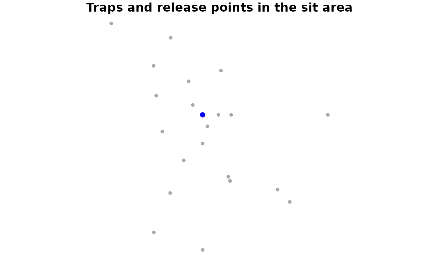
You can make more professional and even interactive maps by
leveraging other R packages of your choice. This is beyond the scope of
sit, but I’ll provide a few examples here using the package tmap. To
learn more on mapping, see the chapter Making maps with
R in Robin Lovelace’s excellent book Geocomputation with
R.
library(tmap)
tmap_cmode <- tmap_mode("view")
#> tmap mode set to interactive viewing
tm_basemap("CartoDB") +
tm_shape(
  sit_traps(sit_prototype, area = "sit", stage = "adult")
) +
  tm_dots() +
  tm_shape(
    sit_revents(sit_prototype, type = "point") %>%
      st_as_sf()
  ) +
  tm_bubbles(
    col = "colour",
    jitter = 1       # Jitter a bit to see the overlapping release points
  )
tmap_mode(tmap_cmode)
#> tmap mode set to plotting
Note how we retrieved only adult traps from the
sit area, and only the point releases, out of
all available traps and releases. We will see how that worked in the
following section.
Extraction functions
Extraction functions allow retrieving the data contained in a
sit object, while filtering specific groups as needed.
Here we describe the list of arguments of each extraction function, with a few examples. This is very much borrowed from the help pages, but focused on the extraction method only.
sit_trap_types()
Arguments:
x
|
A sit object.
|
This one is simple: it only takes a sit object and
returns the list of trap types. E.g.
sit_trap_types(sit_prototype)
#>   id                name label stage description
#> 1  1             Ovitrap   OVT   egg          NA
#> 2  2         BG-Sentinel   BGS adult          NA
#> 3  3 Human Landing Catch   HLC adult          NA
The result is a data.frame itself. Thus, if you really
need to filter some observations, you can put your R-skills to use:
sit_trap_types(sit_prototype) %>%
  dplyr::filter(stage == "egg")
#>   id    name label stage description
#> 1  1 Ovitrap   OVT   egg          NA
sit_traps()
Arguments:
x
|
A sit object.
|
type
|
Character vector. Labels of requested trap types. By default,
sit_trap_types()$label.
|
stage
|
Character vector. Either adult, egg or both
(default).
|
area
|
Character vector. Either control, sit or both
(default).
|
Retrieve the table of ovitraps:
sit_traps(sit_prototype, type = "OVT")
#> Simple feature collection with 21 features and 8 fields (with 21 geometries empty)
#> Geometry type: POINT
#> Dimension:     XY
#> Bounding box:  xmin: NA ymin: NA xmax: NA ymax: NA
#> CRS:           +proj=laea +x_0=0 +y_0=0 +lon_0=16.41472 +lat_0=48.23528
#> First 10 features:
#>    id code area label type_name type_label type_stage type_description
#> 1  22 CS01  sit    NA   Ovitrap        OVT        egg               NA
#> 2  23 CS02  sit    NA   Ovitrap        OVT        egg               NA
#> 3  24 CS03  sit    NA   Ovitrap        OVT        egg               NA
#> 4  25 CS04  sit    NA   Ovitrap        OVT        egg               NA
#> 5  26 CS05  sit    NA   Ovitrap        OVT        egg               NA
#> 6  27 CS06  sit    NA   Ovitrap        OVT        egg               NA
#> 7  28 CS07  sit    NA   Ovitrap        OVT        egg               NA
#> 8  29 CS08  sit    NA   Ovitrap        OVT        egg               NA
#> 9  30 CS09  sit    NA   Ovitrap        OVT        egg               NA
#> 10 31 CS10  sit    NA   Ovitrap        OVT        egg               NA
#>       geometry
#> 1  POINT EMPTY
#> 2  POINT EMPTY
#> 3  POINT EMPTY
#> 4  POINT EMPTY
#> 5  POINT EMPTY
#> 6  POINT EMPTY
#> 7  POINT EMPTY
#> 8  POINT EMPTY
#> 9  POINT EMPTY
#> 10 POINT EMPTY
Note that this coincides with the table of traps for the
stage = 'egg'.
However, traps in the control area are only a
subset:
sit_traps(sit_prototype, area = "control")
#> Simple feature collection with 7 features and 8 fields (with 7 geometries empty)
#> Geometry type: POINT
#> Dimension:     XY
#> Bounding box:  xmin: NA ymin: NA xmax: NA ymax: NA
#> CRS:           +proj=laea +x_0=0 +y_0=0 +lon_0=16.41472 +lat_0=48.23528
#>   id code    area label type_name type_label type_stage
#> 1 36 BL01 control    NA   Ovitrap        OVT        egg
#> 2 37 BL02 control    NA   Ovitrap        OVT        egg
#> 3 38 BL03 control    NA   Ovitrap        OVT        egg
#> 4 39 BL04 control    NA   Ovitrap        OVT        egg
#> 5 40 BL05 control    NA   Ovitrap        OVT        egg
#> 6 41 BL06 control    NA   Ovitrap        OVT        egg
#> 7 42 BL07 control    NA   Ovitrap        OVT        egg
#>   type_description    geometry
#> 1               NA POINT EMPTY
#> 2               NA POINT EMPTY
#> 3               NA POINT EMPTY
#> 4               NA POINT EMPTY
#> 5               NA POINT EMPTY
#> 6               NA POINT EMPTY
#> 7               NA POINT EMPTY
sit_revents()
Arguments:
x
|
A sit object.
|
type
|
Character vector. Which types of release events to
retrieve. Either point or areal or both
(default).
|
sit_revents(sit_prototype, type = 'point')
#>   id  type site_id                date colour     n    geometry
#> 1  1 point       1 2019-11-24 23:00:00 yellow 10000 POINT (0 0)
#> 2  2 point       1 2019-11-30 23:00:00    red 10000 POINT (0 0)
#> 3  3 point       1 2019-12-12 23:00:00   blue 10000 POINT (0 0)
sit_revents(sit_prototype, type = 'areal')
#>   id  type site_id                date colour     n    geometry
#> 1  4 areal       2 2019-12-20 23:00:00   pink 10000 POINT EMPTY
sit_revents(sit_prototype)
#>   id  type site_id                date colour     n    geometry
#> 1  1 point       1 2019-11-24 23:00:00 yellow 10000 POINT (0 0)
#> 2  2 point       1 2019-11-30 23:00:00    red 10000 POINT (0 0)
#> 3  3 point       1 2019-12-12 23:00:00   blue 10000 POINT (0 0)
#> 4  4 areal       2 2019-12-20 23:00:00   pink 10000 POINT EMPTY
sit_adult_surveys() and
sit_egg_surveys()
Extract survey data, possibly filtering results.
Arguments:
x
|
A sit object
|
area
|
Character. Either control, sit or both
(default).
|
trap_type
|
Character. Any of sit_trap_types(x)$label. Typically,
OVT for sit_egg_surveys() and BGS
or HLC for sit_adult_surveys().
|
following_releases
|
A sit_release object with a subset of release events or
missing (default) for all release events. Use in combination with
following_days to filter surveys of the target populations
within a given number of days after release. Note that counts of wild
populations will always be included in the results with
a value of NA in pop_col.
|
following_days
|
Integer or missing (default). Number of days after releases to return,
if following_releases is not missing.
|
species
|
Character or NULL (default). Filter surveys for a particular species, or ignore the species if NULL. |
Retrieve all the egg surveys in the control area:
sit_egg_surveys(sit_prototype, area = "control")
#> # A tibble: 154 × 6
#>       id trap_code datetime_start      datetime_end        fertile     n
#>    <int> <chr>     <dttm>              <dttm>              <lgl>   <dbl>
#>  1   309 BL01      2019-11-21 23:00:00 2019-11-28 23:00:00 TRUE       41
#>  2   310 BL01      2019-11-21 23:00:00 2019-11-28 23:00:00 FALSE      37
#>  3   311 BL02      2019-11-21 23:00:00 2019-11-28 23:00:00 TRUE      102
#>  4   312 BL02      2019-11-21 23:00:00 2019-11-28 23:00:00 FALSE      20
#>  5   313 BL03      2019-11-21 23:00:00 2019-11-28 23:00:00 TRUE      204
#>  6   314 BL03      2019-11-21 23:00:00 2019-11-28 23:00:00 FALSE      18
#>  7   315 BL04      2019-11-21 23:00:00 2019-11-28 23:00:00 TRUE      354
#>  8   316 BL04      2019-11-21 23:00:00 2019-11-28 23:00:00 FALSE      54
#>  9   317 BL05      2019-11-21 23:00:00 2019-11-28 23:00:00 TRUE       31
#> 10   318 BL05      2019-11-21 23:00:00 2019-11-28 23:00:00 FALSE      10
#> # … with 144 more rows
Retrieve the adult surveys from the day that followed the areal release. Only counts from the target release, or the wild population, please.
sit_adult_surveys(
  sit_prototype,
  following_releases = sit_revents(sit_prototype, type = 'areal'),
  following_days = 1
)
#> # A tibble: 63 × 7
#>       id trap_code pop_col datetime_start      datetime_end        sex
#>    <int> <chr>     <chr>   <dttm>              <dttm>              <chr>
#>  1  2227 1         wild    2019-12-20 23:00:00 2019-12-21 23:00:00 fema…
#>  2  2228 1         wild    2019-12-20 23:00:00 2019-12-21 23:00:00 male
#>  3  2232 1         pink    2019-12-20 23:00:00 2019-12-21 23:00:00 male
#>  4  2233 2         wild    2019-12-20 23:00:00 2019-12-21 23:00:00 fema…
#>  5  2234 2         wild    2019-12-20 23:00:00 2019-12-21 23:00:00 male
#>  6  2238 2         pink    2019-12-20 23:00:00 2019-12-21 23:00:00 male
#>  7  2239 3         wild    2019-12-20 23:00:00 2019-12-21 23:00:00 fema…
#>  8  2240 3         wild    2019-12-20 23:00:00 2019-12-21 23:00:00 male
#>  9  2244 3         pink    2019-12-20 23:00:00 2019-12-21 23:00:00 male
#> 10  2245 4         wild    2019-12-20 23:00:00 2019-12-21 23:00:00 fema…
#> # … with 53 more rows, and 1 more variable: n <dbl>
SIT results
1. Descriptive summaries
Dispersal of sterile males in space and time.
## Retrieve age since release date of each survey
sm_ages <- survey_ages(
  surveys  = sit_adult_surveys(sit_prototype),
  releases = sit_revents(sit_prototype, type = 'point')
)

## Summarise counts by trap and age-group (by 5 days)
sm_summary <-
  sm_ages %>%
  mutate(
    age_group = cut(age, 5*(0:6))
  ) %>%
  filter(!is.na(age_group)) %>%   # remove ages 30+ (max is 36)
  group_by(trap_code, age_group) %>%
  summarise(n = sum(n), .groups = 'drop')

## Join this data to the geospatial information of the traps
sm_sf <- sit_traps(sit_prototype, area = "sit", stage = "adult") %>%
  left_join(sm_summary, by = c(code = 'trap_code'))

tm_shape(sm_sf) +
  tm_bubbles(size = 'n') +
  tm_facets(by = 'age_group')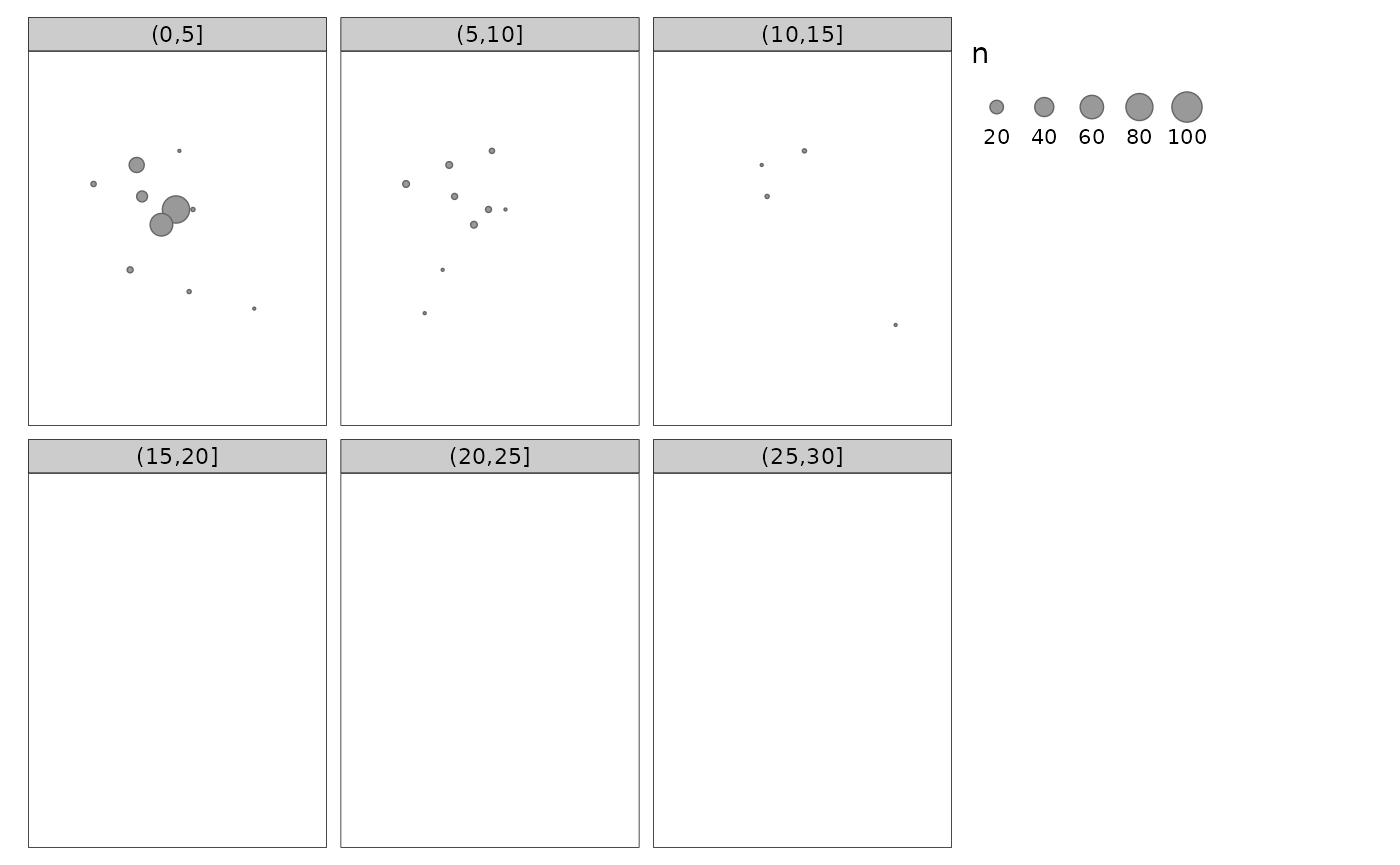
2. Competitiveness
The competitiveness \(\gamma\) of the sterile male individuals is defined as their relative capacity to mate with a wild female, compared to a wild male.
Thus, in a homogeneously mixed population with \(M_s\) sterile males and \(M_w\) wild males, the probability that a mating occurs with a sterile individual is \[ p_s = \frac{\gamma M_s}{M_w + \gamma M_s} = \frac{\gamma R_{sw}}{1 + \gamma R_{sw}}, \] where \(R_{sw} = M_s/M_w\) is the sterile-wild male ratio. At a given sterile-wild male ratio \(R_{sw} = M_s/M_w\) we observe a fertility rate \(H_s\) in the field.
Assuming a residual fertility rate \(H_{rs}\) for sterile males and a natural fertility rate \(H_w\) for wild males, the observed fertility rate \(H_s\) in the field is: \[\begin{equation} H_s = p_s H_{rs} + (1-p_s)H_w = \frac{\gamma R_{sw}}{1 + \gamma R_{sw}} H_{rs} + \frac{1}{1 + \gamma R_{sw}} H_w. \end{equation}\]
Solving the above equation for \(\gamma\) we obtain the Fried index, which estimates the competitiveness based on observed fertility rates and the sterile-wild male ratio: \[\begin{equation} F = \frac{H_w – H_s}{H_s-H_{rs}} \bigg/ R_{sw} \end{equation}\] where \(H_w\) is the percentage egg hatch in the control area (i.e. the natural fertility); \(H_s\) is the percentage egg hatch in the release area (observed fertility under a sterile-wild male ratio \(R_{sw}\)) and \(H_{rs}\) is the residual fertility of sterile males.
This requires the estimation of:
The sterile-wild males ratio \(R_{sw}\). Estimated from the observed ratios in adult surveys in the following 7 days after areal releases by default.
The natural fertility \(H_w\). Estimated from egg-hatching rates in the control area.
The observed fertility in the release area \(H_s\). Estimated from egg-hatching rates in the SIT area.
The residual fertility of sterile males \(H_{rs}\). This depends on the level of radiation used for sterilisation, and the influx of females from beyond the SIT area. This cannot be estimated from SIT data and needs to be fixed by the user. Using \(H_{rs} = 0\) reduces to the so-called CIS index.
sit_competitiveness(sit_prototype, residual_fertility = 0.05)
#>
#> ── Sterile male competitiveness ────────────────────────────────────────
#> ℹ Estimated value: 0.6
#>
#>
#> Component                         Value
#> -------------------------------  ------
#> Sterile-wild male ratio            1.13
#> Natural fertility                  0.84
#> Observed fertility in SIT area     0.52
#> Sterile fertility (assumed)        0.05
If there were more than one areal release, we could compute the
estimated competitiveness for each one separately by specifying
following_release. We can also control the number of days
following the release to be used for the calculation of the sterile-wild
male ratio.
sit_competitiveness(
  sit_prototype,
  following_releases = sit_revents(sit_prototype, type = "areal")[1,],
  following_days = 10,
  residual_fertility = 0.05
)
#>
#> ── Sterile male competitiveness ────────────────────────────────────────
#> ℹ Estimated value: 1.18
#>
#>
#> Component                         Value
#> -------------------------------  ------
#> Sterile-wild male ratio            0.58
#> Natural fertility                  0.84
#> Observed fertility in SIT area     0.52
#> Sterile fertility (assumed)        0.05
We can be shocked by the difference in the estimate after simply widening the observation window to 10 days rather than 7, and legitimately ask which time-span is more appropriate.
Notice that the only component of the calculation that changed sensibly is the sterile-wild male ratio, which essentially halved.
Let’s see how the relationship between captured sterile and wild males evolve in time. We can look at the ratio, but the difference is a more natural scale.
areal_release <- sit_revents(sit_prototype, type = "areal")

areal_surveys <- sit_adult_surveys(
    sit_prototype,
    area = "sit",
    following_releases = areal_release,
    following_days = 10
  )

sterile_wild_male_ratio(areal_surveys) %>%
  mutate(
    age = as.numeric(datetime_end - areal_release$date)
  ) %>%
  group_by(age) %>%
  summarise(
    sterile = sum(sterile),
    wild = sum(wild),
    swdiff = sterile - wild
  ) %>%
  ggplot(aes(age, swdiff)) +
  geom_point() +
  geom_smooth(method = 'loess', formula = 'y ~ x') +
  labs(x = "Age", y = "Sterile - wild difference")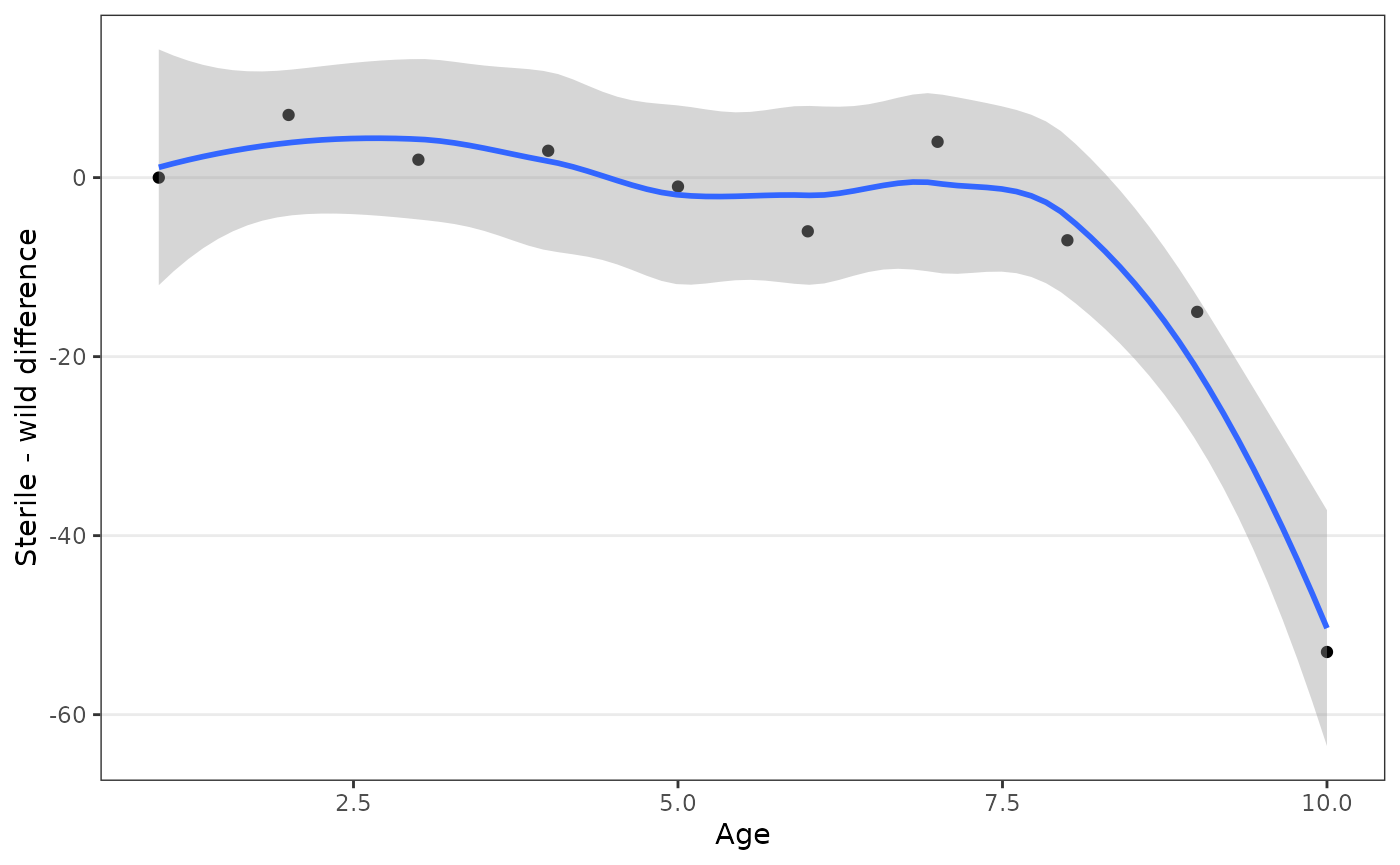
Starting from day 8, the number of captured sterile males drops consistently with respect to the captured wild males, which explains the difference in the estimate of competitiveness.
Since the calculation pools observations assuming a constant ratio, we can conclude that 7 days was an appropriate time-span for these data.
3. Dispersal
Mean Distance Travelled (MDT)
Since the dispersion evolves in time, typically increasing with time since release, we compute the MDT at each day \(j\) and, potentially, for the population corresponding to the release event \(k\).
\[\begin{equation} \text{MDT}_{jk} = \sum_{i = 1}^{n_t} w_{ik}\,n_{ijk}\,d_i \bigg/ \sum_{i = 1}^{n_t} w_{ik}\,n_{ijk} \end{equation}\] where \(n_t\) is the total number of traps, \(d_i\) is the distance from trap \(i\) to the release site of event \(k\) and \(n_{ijk}\) is the number of sterile males surveyed at trap \(i\), in day \(j\) after release event \(k\).
Furthermore, a set of weights \(w_{ik}\) for each trap and release event
can be used, in order to account for a inhomogeneous arrangement of the
traps, as explained below. This is activated by the argument
spatial_adjustment in sit_mdt() and
sit_flight_range(). Without spatial adjustment, the weights
are set as \(w_{ik} = 1\) and the MDT
reduces to the so-called Mean Dispersal Distance (MDD).
Depending on the needs and hypotheses, the calculation could also aggregate observations by days, populations or both.
If most traps were concentrated far away from the release points, then MDT would be artificially inflated as a consequence. A way of correcting for this is to weight the counts by the inverse relative local trap density at each trap. However, a spatial density estimate of traps would be too noisy with only a couple dozen traps and suffer from considerable edge effects. Thus, we assume isotropy (neglect the direction) and consider only the radial density from the release site.
Trap density with respect to the distance from the release point increases linearly with the distance for a uniform distribution of traps.
The relative density is the ratio between the observed density and the expected density under uniformity (straight line). While the \(\omega_i\) is the inverse of the ratio at the distance of the corresponding trap (Figure below).

This approach also suffers from edge effect. However, the trick to solve it is much simpler and the results more robust. The figure above shows the uncorrected density in grey and the adjusted density as a black curve with points at the observed distances.
The only issue would be for trap patterns that are strongly concentrated in specific directions at different distances. However, this seems unlikely.
With this spatial adjustment (performed by default), we can assess the MDT by each released population (point releases only), and we can also plot the histogram of travelled distances weighted by the number of observations and the spatial adjustment:
(mdt_prototype <- sit_mdt(sit_prototype, by = "population"))
#>
#> ── Mean Distance Travelled ─────────────────────────────────────────────
#>
#>
#> population       mdt
#> -----------  -------
#> blue          110.08
#> red            63.48
#> yellow         69.35
plot(mdt_prototype)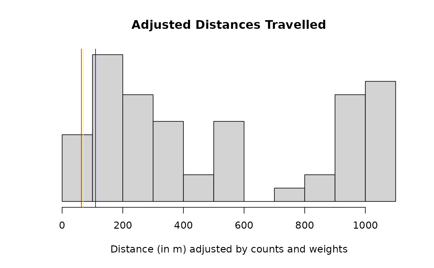
The histogram excludes the most extreme 2.5 % of observations on each side, to improve visualisation. The vertical lines display the mean distances travelled by population. They appear shifted towards 0 due to a large number of adjusted distances near 0 that are not shown.
Contrast with the results without the spatial adjustment. The estimated distances are shorter, due to a over-represented number of traps at shorter distances.
sit_mdt(sit_prototype, by = "population", spatial_adjustment = FALSE)
#>
#> ── Mean Distance Travelled ─────────────────────────────────────────────
#>
#>
#> population      mdt
#> -----------  ------
#> blue          66.97
#> red           52.44
#> yellow        58.67
We can also consider the MDT by age (pooling across populations).
sit_mdt(sit_prototype, by = "age")
#>
#> ── Mean Distance Travelled ─────────────────────────────────────────────
#>
#>
#>  age      mdt
#> ----  -------
#>    1    88.39
#>    2    51.75
#>    3    57.35
#>    4    68.11
#>    5   109.28
#>    6    79.75
#>    7   154.33
#>    8    79.38
#>    9   104.39
#>   10   128.51
#>   11   128.51
#>   12    37.38
#>   13   330.73
#>   14   128.51
#>   15    76.27
There is no obvious increase of MDT with time. It could be one particular population which is distorting the results, but we don’t have enough observations to split the MDT by age and population.
On the other hand, estimates get noisier for larger ages since observations are more scarce. If we restricted the analysis to the first 10 days of age, the pattern is more apparent.
sit_mdt(sit_prototype, by = "age") %>%
  filter(age <= 10) %>%
  ggplot(aes(age, mdt)) +
  geom_point() +
  geom_smooth(method = "lm", formula = 'y ~ x')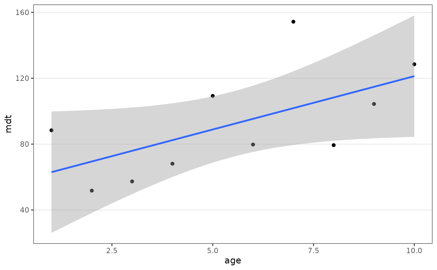
Flight Range
This is an alternative measure of the dispersal capacity of sterile males based on quantiles rather than averages.
The method regresses the log-distances (\(+1\) to avoid divergence) from the release
point as a function of the cumulative (trap-density adjusted) catches.
This relationship is modelled linearly, and the expected distances at
the 50 and 90% adjusted catches with respect to the total are defined as
the corresponding flight ranges FR50 and
FR90.
The function sit_flight_range() uses the levels 50 and
90 by default and allows making a basic plot of the underlying model for
verification.
(fr_prototype <- sit_flight_range(sit_prototype))
#>
#> ── Flight range ────────────────────────────────────────────────────────
#>
#>
#> population    level   cum_adj_catch       FR
#> -----------  ------  --------------  -------
#> blue             50           15.92    73.54
#> blue             90           28.66   240.57
#> red              50           11.63    51.89
#> red              90           20.93   165.90
#> yellow           50            9.13    64.86
#> yellow           90           16.44   172.20
fr_plot <- plot(fr_prototype)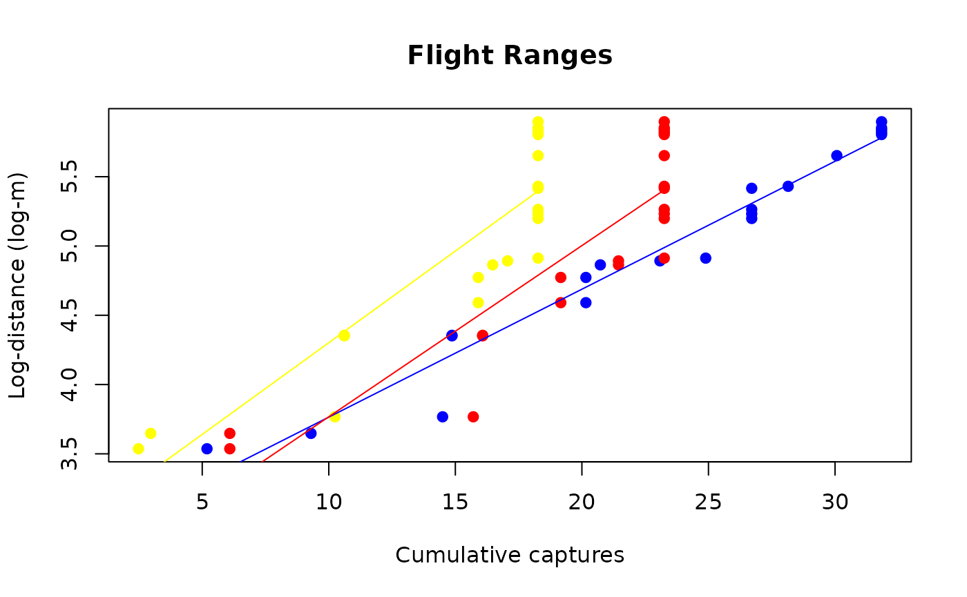
Moreover, the plot method returns the underlying data
invisibly, which allows making a more customised figure. E.g.
fr_plot %>%
  ggplot(aes(cx, logd, colour = population)) +
  geom_point(show.legend = FALSE) +
  geom_smooth(method = "lm", formula = y ~ x, se = FALSE, show.legend = FALSE) +
  labs(x = "Cumulative captures", y = "Log-distance (log-m)") +
  scale_colour_manual(values = unique(fr_plot$population))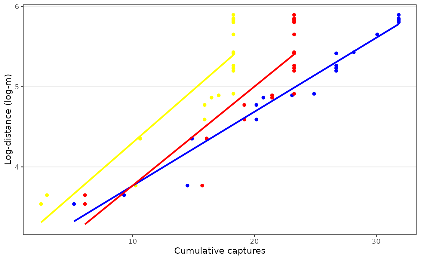
The function also allows defining any number of quantiles and gives results either disaggregated by population (default) or all populations pooled together.
sit_flight_range(sit_prototype, levels = c(25, 50, 75), pool = TRUE)
#>
#> ── Flight range ────────────────────────────────────────────────────────
#>
#>
#> population    level   cum_adj_catch       FR
#> -----------  ------  --------------  -------
#> pooled           25           18.34    29.31
#> pooled           50           36.68    61.46
#> pooled           75           55.02   127.70
Diffusion
Assuming that mosquitoes fly randomly (Brownian motion), their dispersion follow Fick’s first law of diffusion, which postulates that flux goes from regions of high concentration to regions of low concentration, with a magnitude that is proportional to the concentration gradient (spatial derivative). The proportionality constant is the diffusivity \(D\) and depend of the species’ behaviour for that location, season and weather conditions.
Under this model, the Mean Squared Displacement (MSD) of mosquitoes from their release point at time \(t\) is \[ \text{MSD}(t) = 4Dt. \]
From which we can solve for the Diffusion coefficient by using the distances from the release point at which sterile males were captured to estimate the MSD at a given age.
The function sit_diffusion() computes the MSD of the
individuals (by population, by default, or possibly pooling populations)
at the different observed ages, and derives \(D\) as the regression slope. The resulting
object can be plotted to see the underlying regression model.
(diff_prototype <- sit_diffusion(sit_prototype))
#>
#> ── Diffusion coefficient ───────────────────────────────────────────────
#>
#>
#> population      Dest
#> -----------  -------
#> blue          860.72
#> red           139.33
#> yellow        173.71
plot(diff_prototype)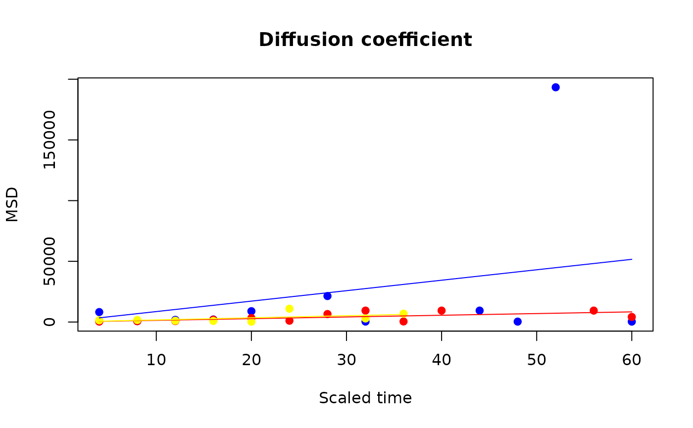
4. Survival
We assume that for a released population of sterile males there is a certain probability of daily survival (\(\pi_\text{PDS}\)), which represents the probability that an individual (or the proportion of individuals that) makes it to the next day.
The proportion \(p_j\) of sterile males still alive at day \(j\) decreases geometrically, starting from some initial survival \(p_0\) at day 0:
\[ p_j = p_0 \, \pi_\text{PDS}^j. \]
Assuming that each day \(j\) we capture a fraction \(c\) of the released individuals that remain alive, we have that the expected number of surveyed individuals at day \(j\) is
\[ E[y_j] = c\, p_0 \, \pi_\text{PDS}^j. \]
In log-scale, \[ \log(E[y_j]) = \alpha + \beta \cdot j, \] where \(\alpha = \log(c\, p_0)\) and \(\beta = \log(\pi_\text{PDS})\).
This leads to estimating PDS by regressing the log-number of catches (+ 1, to avoid divergences) on the number of days since release (age).
The methodology was taken from Kay and Muir (1998), but originally developed in Gillies (1961). There is no appropriate statistical model other than the observation the the rate of decrease in the caught individuals is approximately constant, which leads to the regression approach.
The recapture \(\theta\) and survival \(S\) rates are computed as
\[\begin{equation} \begin{aligned} \theta & = \exp(\alpha) / (N + \exp(\alpha)) \\ S & = \exp(\beta) / (1 + \theta)^{1/d}, \end{aligned} \end{equation}\] where \(\alpha\) and \(\beta\) are the regression coefficients of the log-catches against age, \(N\) is the number of individuals released and \(d\) is the number of days after release (age in days). We use \(d = 1\).
The function sit_survival() returns a table with the
Probability of Daily Survival (PDS), the Average Life
Expectancy ALE, Recapture Rate
RR, Survival Rate SR), by population
(by default, unless pool = TRUE)
(surv_prototype <- sit_survival(sit_prototype))
#>
#> ── Survival ────────────────────────────────────────────────────────────
#>
#>
#> population    N_released    PDS    ALE   RRx1e3     SR
#> -----------  -----------  -----  -----  -------  -----
#> blue               10000   0.81   4.83     1.96   0.81
#> red                10000   0.81   4.83     1.76   0.82
#> yellow             10000   0.81   4.83     1.38   0.82
plot(surv_prototype)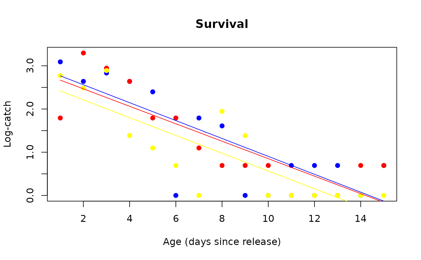
5. Density or size of the wild population
An estimation of the density, or equivalently, the size of the wild mosquito population is necessary for the determination of the appropriate quantity of sterile males to be released for controlling the population effectively.
A simple estimate is obtained as follows (Thompson 2012, Ch. 18). Let the total captures at a day \(t\) be the sum of \(m_t\) marked and \(n_t\) wild mosquitoes. Assuming that the proportion of marked individuals in the sample equals that in the population of size \(P\): \[ \frac{m_t}{m_t + n_t} = \frac{M_t}{M_t + P}, \] where \(M_t = R\,S^{a_t}\) is the number of marked individuals captured at time \(t\), with \(R\) the number of released adults, \(S\) the daily survival rate and \(a_t\) the number of days since release (age). I.e., the number of marked individuals at time \(t\) is the remaining number from those released that survived for \(a_t\) days.
The Lincoln Index (a.k.a. the Petersen estimator) has been used as a simple estimate of the wild male population size, assuming that the survival rate of an individual remains constant. Here we use a modified version that corrects for small samples and compensates for daily survival. \[ P_t = R\,S^{a_t}\,(n_t + 1) / (m_t + 1). \]
The values of \(R\), \(n_t\), \(m_t\) and \(t\) can be gathered from the adult surveys data. The calculation requires the estimation of the survival rate \(S\).
This provides multiple estimates of the population size, one for each age \(t\) and for each released population, which can be averaged to compute a final estimate based on all the available data.
The calculation needs to be split by released population. First, because survival rates could be different among populations, but also because the number \(n_t\) of captured wild males at a given date can be compared against the number of captured sterile males \(m_t\) at different ages. Still, the function allows pooling data across population as if they were the same.
The function returns a point estimate and the standard deviation.
sit_wild_size(sit_prototype)
#>
#> ── Wild male population size ───────────────────────────────────────────
#>
#>
#> population      p_est      p_sd
#> -----------  --------  --------
#> blue          4981.57   5420.85
#> red           3471.37   1919.16
#> yellow        6527.88   4248.72