Getting Started
sit.Rmd
library(dplyr)  # Data manipulation
library(tidyr)  # Tidy data
library(sf)     # Simple features for R (spatial objects)
library(sit)    # Analyse MRR data from SIT experiments
Overview
The purpose of sit is to help analyse
mark-release-recapture (MRR) data from sterile insect technique (SIT)
field experiments.
There are two basic stages in any analysis:
Importing data into
sitRetrieving results from
sit
Here, we will quickly review some concepts needed to work with
sit while going through a fictitious case study. Links to
more detailed materials will be provided along the way.
Data model
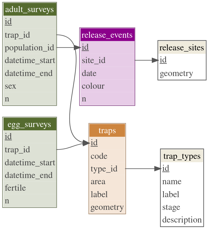
Data model diagram.
The main concepts involved in a MRR SIT experiment are represented in the Figure above and can be summarised as follows:
Sterile male mosquitoes are released in a release
event. Relevant properties are: the number of released
individuals, n, the dye colour use for
identification, the date and time of release and the
release site.
Release sites can be either points or the
whole study area (in the case of areal/line releases). In the
former case, release sites have a geometry represented by
spatial coordinates, while in the latter case the geometry
is empty.
The relationship between release_events and
release_sites implies that there can be any number of
release events from the same site.
Mosquitoes (both sterile and wild) are subsequently captured in adult
traps. Relevant properties are: their location (point
geometry), the area (study or
control) and a identification code as used in the
field. Furthermore, wild females lay their eggs in another type of
traps (ovitraps).
Both adult and egg traps can be of different types,
which is why each trap is associated with a specific trap
type. Properties of trap types are: its full name
(e.g. BG-Sentinel) and a shorter label
(e.g. BGS), the target stage (adult or egg)
and an optional description.
Finally, traps are regularly surveyed in order to
collect the experimental data. Both adult and egg surveys record the
surveyed trap and the period of capture. Adult surveys
also record the population_id of the captured individuals
(either wild or the colour of one of the released
populations), their sex and the total number n
of individuals of each group. Egg surveys instead,
record the number of eggs which were fertile or not.
Package organisation
First, load the package as follows:
The package provides a series of functions to import data and to retrieve results.
All functions in the package are prefixed by sit_. This
is convenient for finding function names in combination with the
auto-complete feature that is provided by most development
environments such as RStudio or VSCode.
The typical workflow is as follows:
Import data tables from files (
.csv,.xls(x), …) into Rdata.frames.-
Transform and reshape the data into the structures required by import functions in
sit. Here is a list of the mainsitfunctions used at this stage:Import functions. Function Description sit_revents()Import release events and sites. sit_traps()Import traps sit_adult_surveys()Import adult surveys sit_egg_surveys()Import egg surveys sit()Gather data about traps, release events and field survey data into a sitobject. Gather all the data (traps, releases, surveys) into a
sitobject.Query the
sitobject to verify that everything was correctly interpreted.-
Retrieve results from the
sitobject. A list of relevantsitfunctions is shown below:Estimating functions. Function Description sit_competitiveness()Competitiveness of sterile males sit_mdt()Mean Distance Travelled (MDT) sit_flight_range()Flight Range sit_diffusion()Diffusion coefficient sit_survival()Survival statistics sit_wild_size()Size of the wild male population
Introductory example
This section will skim through a complete analysis. Most details will
be deferred to more specific articles. The objective is to quickly
acquire a perspective of the general workflow. See
vignette("importing", package = "sit") for specific details
on the format and structure required by the import functions.
The package provides some realistic but fictitious data files that
can be located with system.file(). Specifically:
list.files(system.file("extdata", package = "sit"))
#> [1] "adult_surveys.csv"         "bgs_traps_coordinates.csv"
#> [3] "egg_surveys.csv"           "releases.csv"
1. Read data tables into R
releases_raw <- read.csv(
  system.file("extdata/releases.csv", package = "sit")
)

bgs_traps_raw <- read.csv(
  system.file("extdata/bgs_traps_coordinates.csv", package = "sit")
)

adults_raw <- read.csv(
  system.file("extdata/adult_surveys.csv", package = "sit")
)

eggs_raw <- read.csv(
  system.file("extdata/egg_surveys.csv", package = "sit")
)
2. Transform raw data
This step will require some basic skills of data-manipulation in R.
An accessible introduction to what we’ll use can be found in the Introduction
to dplyr and tidyr’s tutorial on Pivoting.
The raw data of release events have geographical coordinates for the point releases. There is also one areal release with missing coordinates.
head(releases_raw)
#>         date colour     n      lon      lat
#> 1 2019-11-25 yellow 10000 16.41472 48.23528
#> 2 2019-12-01    red 10000 16.41472 48.23528
#> 3 2019-12-13   blue 10000 16.41472 48.23528
#> 4 2019-12-21   pink 10000       NA       NA
The former need to be transformed into a spatial object of POINT
features (using the package
sf), while the areal release is treated separately.
## Point releases
p_releases <- releases_raw %>%
  dplyr::filter(!is.na(lon)) %>%      # Observations with non-missing coords
  st_as_sf(                           # Convert to spatial
    coords = c("lon", "lat"),           # Variables with coordinates
    crs = 4326                          # Code for GPS coordinates
  )
#> Simple feature collection with 3 features and 3 fields
#> Geometry type: POINT
#> Dimension: XY
#> Bounding box: xmin: 16.41472 ymin: 48.23528 xmax: 16.41472 ymax: 48.23528
#> Geodetic CRS: WGS 84
#> date colour n geometry
#> 1 2019-11-25 yellow 10000 POINT (16.41472 48.23528)
#> 2 2019-12-01 red 10000 POINT (16.41472 48.23528)
#> 3 2019-12-13 blue 10000 POINT (16.41472 48.23528)
## Areal release
a_releases <- releases_raw %>%
  dplyr::filter(is.na(lon)) %>%    # Observations with missing coords
  dplyr::select(-lon, -lat)        # Select variables (to remove)
#> date colour n
#> 1 2019-12-21 pink 10000Combine point and areal releases
using c().
ix_releases <- c(sit_revents(p_releases), sit_revents(a_releases))The traps data file contains only an id and GPS coordinates. The file name indicates they are BGS traps (a type of adult traps). We have to know (e.g. from project documentation) that they are located in the study area.
head(bgs_traps_raw)
#>   id      lon      lat
#> 1  1 16.41295 48.23646
#> 2  2 16.41304 48.23574
#> 3  3 16.41326 48.23488
#> 4  4 16.41529 48.23528
#> 5  5 16.41538 48.23635
#> 6  6 16.41422 48.23609
We need to transform the object into a spatial object of POINT
features (using the package
sf), and add some of the missing variables.
a_traps <- bgs_traps_raw %>%
  mutate(                         # Modify (add) variables
    type = "BGS",
    area = "sit"
  ) %>%
  st_as_sf(                       # Convert to spatial
    coords = c("lon", "lat"),         # Variables with coordinates
    crs = 4326                        # Code for GPS coordinates
  )
Note that declaring type = 'BGS' implies that these
traps target the adult stage, since:
sit_trap_types()
#>   id                name label stage description
#> 1  1             Ovitrap   OVT   egg          NA
#> 2  2         BG-Sentinel   BGS adult          NA
#> 3  3 Human Landing Catch   HLC adult          NA
Furthermore, there are 14 ovitraps in the study area and 7 more in a
control area, although there is no data file for these, since
coordinates are not strictly required (albeit recommended). We declare
these simply by passing a vector of trap codes, the area and a
valid type to sit_traps(). Finally, we combine
(c()) all trap types together into a single object.
ix_traps <- c(
  sit_traps(a_traps),
  sit_traps(sprintf("CS%02d", 1:14), area = 'sit', type = 'OVT'),
  sit_traps(sprintf("BL%02d", 1:7), area = 'control', type = 'OVT')
)
Survey data of adult traps have been collected across multiple columns.
head(adults_raw)
#>   trap     survey wild_female wild_male yellow_male red_male blue_male
#> 1    1 2019-11-26           0         0           0       NA        NA
#> 2    2 2019-11-26           0         0           0       NA        NA
#> 3    3 2019-11-26           2         1           0       NA        NA
#> 4    4 2019-11-26           0         0          10       NA        NA
#> 5    5 2019-11-26           0         0           0       NA        NA
#> 6    6 2019-11-26           0         2           4       NA        NA
#>   pink_male
#> 1        NA
#> 2        NA
#> 3        NA
#> 4        NA
#> 5        NA
#> 6        NA
We need to reshape (pivot) the table to make it tidy (one variable per column) and add the implicit information about the duration of each survey (1 day).
(
  adult_surveys <-
    adults_raw %>%
    ## Reshape into long format
    pivot_longer(
      cols = wild_female:pink_male,
      names_to = "pop_sex",
      values_to = "n"
    ) %>%
    ## Separate variables
    separate(
      pop_sex,
      into = c("population", "sex"),
      sep = "_"
    ) %>%
    ## Include the missing duration of the sampling period
    mutate(
      duration = 1
    )
)
#> # A tibble: 4,536 × 6
#>     trap survey     population sex        n duration
#>    <int> <chr>      <chr>      <chr>  <int>    <dbl>
#>  1     1 2019-11-26 wild       female     0        1
#>  2     1 2019-11-26 wild       male       0        1
#>  3     1 2019-11-26 yellow     male       0        1
#>  4     1 2019-11-26 red        male      NA        1
#>  5     1 2019-11-26 blue       male      NA        1
#>  6     1 2019-11-26 pink       male      NA        1
#>  7     2 2019-11-26 wild       female     0        1
#>  8     2 2019-11-26 wild       male       0        1
#>  9     2 2019-11-26 yellow     male       0        1
#> 10     2 2019-11-26 red        male      NA        1
#> # … with 4,526 more rows
ix_adults <- sit_adult_surveys(adult_surveys)We have a similar situation with egg surveys:
head(eggs_raw)
#>   trap     survey fertile sterile
#> 1 CS01 2019-11-29      23       2
#> 2 CS02 2019-11-29     156      20
#> 3 CS03 2019-11-29     160     135
#> 4 CS04 2019-11-29      13       8
#> 5 CS05 2019-11-29     119     102
#> 6 CS06 2019-11-29       1       0
egg_surveys <-
  eggs_raw %>%
  ## Reshape into long format and convert the hatched
  ## status into a logical variable.
  pivot_longer(
    cols = fertile:sterile,
    names_to = "fertile",
    names_transform = list(
      fertile = function(.) {. == "fertile"}  # makes it logical
    ),
    values_to = "n"
  ) %>%
  ## Include the missing duration of the sampling period
  mutate(
    duration = 7
  )
ix_eggs <- sit_egg_surveys(egg_surveys)3. Build the sit object.
Finally, integrate all the data about release events, traps and
surveys into a sit object, using the function of the same
name:
ix_sit <- sit(
  traps          = ix_traps,
  release_events = ix_releases,
  adult_surveys  = ix_adults,
  egg_surveys    = ix_eggs
)
This object that we have just built is (almost) identical to the data
set sit_prototype provided by the package. The only
difference is the coordinate reference
system used.
Thus, for testing the package, you can directly use
sit_prototype which is a fully specified sit
object, and skip the importing operations entirely.
4. Query the sit object
Various standard methods allow you to verify that everything was
correctly interpreted, whereas more specific methods let you retrieve
the data from the sit object.
Printing the sit object provides a short
numerical overview of the data it contains:
print(ix_sit)
#> ── sit ─────────────────────────────────────────────────────────────────
#> Release events: 1 (areal) + 3 (point)
#> Release sites : 2
#> Adult traps   : 21 (sit)
#> Egg traps     : 7 (control) + 14 (sit)
#> Trap types    : 21 (BGS) + 21 (OVT)
#> Surveys       : 3486 (adult) + 462 (egg)
# ix_sit         # Same
More detailed information about the sit object can be
retrieved using other generic methods. See Retrieving results.
The same functions used for importing traps
(sit_traps()), release events (sit_revents())
and surveys (sit_adult_surveys and
sit_egg_surveys()) also work as extractors of the
corresponding data from a sit object.
sit_revents(ix_sit)
#>   id  type site_id       date colour     n                  geometry
#> 1  1 point       1 2019-11-25 yellow 10000 POINT (16.41472 48.23528)
#> 2  2 point       1 2019-12-01    red 10000 POINT (16.41472 48.23528)
#> 3  3 point       1 2019-12-13   blue 10000 POINT (16.41472 48.23528)
#> 4  4 areal       2 2019-12-21   pink 10000               POINT EMPTY
sit_traps(ix_sit)
#> Simple feature collection with 42 features and 8 fields (with 21 geometries empty)
#> Geometry type: POINT
#> Dimension:     XY
#> Bounding box:  xmin: 16.41142 ymin: 48.23202 xmax: 16.41924 ymax: 48.23749
#> Geodetic CRS:  WGS 84
#> First 10 features:
#>    id code area label   type_name type_label type_stage
#> 1   1    1  sit    NA BG-Sentinel        BGS      adult
#> 2   2    2  sit    NA BG-Sentinel        BGS      adult
#> 3   3    3  sit    NA BG-Sentinel        BGS      adult
#> 4   4    4  sit    NA BG-Sentinel        BGS      adult
#> 5   5    5  sit    NA BG-Sentinel        BGS      adult
#> 6   6    6  sit    NA BG-Sentinel        BGS      adult
#> 7   7    7  sit    NA BG-Sentinel        BGS      adult
#> 8   8    8  sit    NA BG-Sentinel        BGS      adult
#> 9   9    9  sit    NA BG-Sentinel        BGS      adult
#> 10 10   10  sit    NA BG-Sentinel        BGS      adult
#>    type_description                  geometry
#> 1                NA POINT (16.41295 48.23646)
#> 2                NA POINT (16.41304 48.23574)
#> 3                NA POINT (16.41326 48.23488)
#> 4                NA POINT (16.41529 48.23528)
#> 5                NA POINT (16.41538 48.23635)
#> 6                NA POINT (16.41422 48.23609)
#> 7                NA   POINT (16.41489 48.235)
#> 8                NA POINT (16.41472 48.23459)
#> 9                NA POINT (16.41571 48.23368)
#> 10               NA POINT (16.41472 48.23202)
sit_adult_surveys(ix_sit)
#> # A tibble: 3,486 × 7
#>       id trap_code pop_col datetime_start      datetime_end        sex
#>    <int> <chr>     <chr>   <dttm>              <dttm>              <chr>
#>  1     1 1         wild    2019-11-25 00:00:00 2019-11-26 00:00:00 fema…
#>  2     2 1         wild    2019-11-25 00:00:00 2019-11-26 00:00:00 male
#>  3     3 1         yellow  2019-11-25 00:00:00 2019-11-26 00:00:00 male
#>  4     4 2         wild    2019-11-25 00:00:00 2019-11-26 00:00:00 fema…
#>  5     5 2         wild    2019-11-25 00:00:00 2019-11-26 00:00:00 male
#>  6     6 2         yellow  2019-11-25 00:00:00 2019-11-26 00:00:00 male
#>  7     7 3         wild    2019-11-25 00:00:00 2019-11-26 00:00:00 fema…
#>  8     8 3         wild    2019-11-25 00:00:00 2019-11-26 00:00:00 male
#>  9     9 3         yellow  2019-11-25 00:00:00 2019-11-26 00:00:00 male
#> 10    10 4         wild    2019-11-25 00:00:00 2019-11-26 00:00:00 fema…
#> # … with 3,476 more rows, and 1 more variable: n <int>
sit_egg_surveys(ix_sit)
#> # A tibble: 462 × 6
#>       id trap_code datetime_start      datetime_end        fertile     n
#>    <int> <chr>     <dttm>              <dttm>              <lgl>   <int>
#>  1     1 CS01      2019-11-22 00:00:00 2019-11-29 00:00:00 TRUE       23
#>  2     2 CS01      2019-11-22 00:00:00 2019-11-29 00:00:00 FALSE       2
#>  3     3 CS02      2019-11-22 00:00:00 2019-11-29 00:00:00 TRUE      156
#>  4     4 CS02      2019-11-22 00:00:00 2019-11-29 00:00:00 FALSE      20
#>  5     5 CS03      2019-11-22 00:00:00 2019-11-29 00:00:00 TRUE      160
#>  6     6 CS03      2019-11-22 00:00:00 2019-11-29 00:00:00 FALSE     135
#>  7     7 CS04      2019-11-22 00:00:00 2019-11-29 00:00:00 TRUE       13
#>  8     8 CS04      2019-11-22 00:00:00 2019-11-29 00:00:00 FALSE       8
#>  9     9 CS05      2019-11-22 00:00:00 2019-11-29 00:00:00 TRUE      119
#> 10    10 CS05      2019-11-22 00:00:00 2019-11-29 00:00:00 FALSE     102
#> # … with 452 more rows
5. Retrieve results from the sit
object.
The main objective of the package is to facilitate the estimation of relevant quantities concerning the competitiveness of sterile male, their dispersal dynamics, their survival rates and the size of the wild male population.
See the vignette Retrieving Results and the reference documentation for more details about all the options for using these functions.
sit_competitiveness(ix_sit)
#>
#> ── Sterile male competitiveness ────────────────────────────────────────
#> ℹ Estimated value: 0.55
#>
#>
#> Component                         Value
#> -------------------------------  ------
#> Sterile-wild male ratio            1.13
#> Natural fertility                  0.84
#> Observed fertility in SIT area     0.52
#> Sterile fertility (assumed)        0.01
sit_mdt(ix_sit, by = "population")
#>
#> ── Mean Distance Travelled ─────────────────────────────────────────────
#>
#>
#> population       mdt
#> -----------  -------
#> blue          110.06
#> red            63.40
#> yellow         69.27
sit_mdt(ix_sit, by = "age")
#>
#> ── Mean Distance Travelled ─────────────────────────────────────────────
#>
#>
#>  age      mdt
#> ----  -------
#>    1    88.31
#>    2    51.68
#>    3    57.30
#>    4    68.00
#>    5   109.24
#>    6    79.60
#>    7   154.17
#>    8    79.34
#>    9   104.23
#>   10   128.45
#>   11   128.45
#>   12    37.32
#>   13   330.24
#>   14   128.45
#>   15    76.24
sit_flight_range(ix_sit)
#>
#> ── Flight range ────────────────────────────────────────────────────────
#>
#>
#> population    level   cum_adj_catch       FR
#> -----------  ------  --------------  -------
#> blue             50           15.89    73.51
#> blue             90           28.60   240.43
#> red              50           11.60    51.82
#> red              90           20.87   165.71
#> yellow           50            9.11    64.78
#> yellow           90           16.40   172.01
sit_diffusion(ix_sit)
#>
#> ── Diffusion coefficient ───────────────────────────────────────────────
#>
#>
#> population      Dest
#> -----------  -------
#> blue          860.67
#> red           138.92
#> yellow        172.64
sit_survival(ix_sit)
#>
#> ── Survival ────────────────────────────────────────────────────────────
#>
#>
#> population    N_released    PDS    ALE   RRx1e3     SR
#> -----------  -----------  -----  -----  -------  -----
#> blue               10000   0.81   4.83     1.96   0.81
#> red                10000   0.81   4.83     1.76   0.82
#> yellow             10000   0.81   4.83     1.38   0.82
sit_wild_size(ix_sit)
#>
#> ── Wild male population size ───────────────────────────────────────────
#>
#>
#> population      p_est      p_sd
#> -----------  --------  --------
#> blue          4981.57   5420.85
#> red           3471.37   1919.16
#> yellow        6527.88   4248.72
Saving and loading
Once you have your data imported as a sit object, you
might want to save it for back up, for continuing work at a later time
without having to re-import the original data from scratch, for sharing
the sit object with someone else, etc.
R provides saving and loading mechanisms for any R object as follows:
## Rather than a temporary file, you might want to define a file name in your
## working directory (`getwd()`) or somewhere else as a character string.
## Use the conventional extension `rds`. E.g.
## my_file <- 'C:/work/project/my_sit.rds'
my_file <- tempfile()
saveRDS(ix_sit, file = my_file)
new_sit <- readRDS(my_file)
identical(new_sit, ix_sit)
#> [1] TRUE
Reproducing results
Beyond saving the sit object with the experimental data,
it is also a good idea to save the analyses and the
results, rather than copying them over to a document and then forgetting
how they were computed.
Working with R is very convenient, since you can simply save the
script that produces all the results. A R
script is just a text file (with conventional extension
.R) with the sequence of commands and function calls that
perform the desired analysis.
Should you want to check where does a result come from, you simply need to look in the script, which is self-documenting. This makes it (almost) trivial to reproduce the results. Either by you or by someone else. In all justice, issues often arise due to differences in the underlying environment (package versions, platform, etc.). However, it is a good start.
An even better approach is to code the analysis report entirely. Making the analysis (e.g. with a R script) and then transferring results (e.g. copying-and-pasting) to a manuscript in separate steps is error-prone and difficult to keep in sync as (inevitably) the calculations get updated and corrected. Instead, we can write the manuscript with the code required to produce the results, all in a single document, which is then compiled into a report.
This approach is called Literate Programming and is not precisely new: it was introduced by Donald Knuth back in 1984. In R, a popular implementation of this idea is R Markdown. It is, by the way, how this document has been produced.
RStudio integrates R Markdown in its interface, which makes it very
easy to get started. Go to
File > New File > R Markdown... and follow the
instructions. Otherwise, you can write a R Markdown file (which is a
text file with a conventional extension .Rmd) and
render the compiled report using
rmarkdown::render().
A final recommendation. Keep all the files (data, code, docs, reports) from a data project organised within a directory. If you use RStudio, setting up a RStudio project in that directory to facilitates switching to and out of it quickly and sharing projects across computers and people.
Some useful references for more insight:
- Hadley Wickham and Garrett Grolemund (2017) R for Data
Science.
- Chapter 8: Workflow: projects. https://r4ds.had.co.nz/workflow-projects.html.
- Chapter 27: R Markdown. https://r4ds.had.co.nz/r-markdown.html
- Rafael A. Irizarry (2021)Introduction to Data Science. Chapter 40: Reproducible projects with RStudio and R markdown. https://rafalab.github.io/dsbook/reproducible-projects-with-rstudio-and-r-markdown.html