Analyse mark-release-recapture data from Sterile Insect Technique (SIT) field experiments
Overview
sit is a R-package currently on active development, after a thorough analysis of requirements.
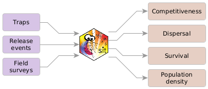
Import data about traps, release events and field surveys into a sit object. Then, query the sit object for estimates of competitiveness, dispersal, survival and wild-population density.
sit outline
Example
First, you need to load the package.
We use some fake data for demonstration purposes. See ?fake_sit.
-
Trap data: set up a
sftable of points with trap coordinates (see,st_as_sf(), for instance), identification code, type (seesit_trap_types()) and area (sit/control). Usesit_traps()to import into asit_trapsobject.fake_traps #> Simple feature collection with 5 features and 3 fields #> Geometry type: POINT #> Dimension: XY #> Bounding box: xmin: -1 ymin: -1 xmax: 2 ymax: 2 #> CRS: NA #> id type area geometry #> 1 a OVT sit POINT (1 1) #> 2 b BGS sit POINT (2 1) #> 3 c HLC sit POINT (1 2) #> 4 d BGS sit POINT (2 2) #> 5 e OVT control POINT (-1 -1)my_traps <- sit_traps(fake_traps) -
Release events: releases can be performed from a single point or homogeneously over the sit area. Set up a table with release dates, colour and number of individuals. For point releases include release coordinates and make it a
sfobject. Lacking geographical coordinates,sitwill interpret it as a areal release.fake_rpoints #> Simple feature collection with 3 features and 3 fields #> Geometry type: POINT #> Dimension: XY #> Bounding box: xmin: 1 ymin: 1 xmax: 2 ymax: 2 #> CRS: NA #> date colour n geometry #> 1 2019-11-25 yellow 10000 POINT (1 2) #> 2 2019-12-01 red 10000 POINT (2 1) #> 3 2019-12-13 blue 10000 POINT (1 2)fake_rareal #> date colour n #> 1 2019-12-21 pink 1000 #> 2 2020-01-09 purple 1000Use
sit_revents()to import intosit_reventsobjects and combine different release types into a singlesit_reventsobject withc().my_releases <- c( sit_revents(fake_rpoints), sit_revents(fake_rareal) ) -
Field survey data: field data are collected at
adultoreggstages of development, depending on the trap type (seesit_trap_types())Field data from adult surveys can be imported using
sit_adult_surveys()from a table such as:fake_adults #> trap survey duration population species sex n #> 1 b 2019-12-16 7 blue aeg male 10 #> 2 d 2019-11-27 7 yellow aeg male 20 #> 3 c 2019-11-27 7 wild aeg female 30 #> 4 d 2019-12-25 7 pink aeg male 40 #> 5 d 2019-12-25 7 wild aeg male 50my_asurveys <- sit_adult_surveys(fake_adults)Field data from egg surveys, include other information such as the hatching rate:
fake_eggs
#>   trap     survey duration fertile  n
#> 1    a 2019-12-01        7    TRUE 15
#> 2    a 2019-12-22        7   FALSE 30
#> 3    a 2019-12-22        7    TRUE 45
#> 4    e 2019-11-15        7    TRUE 60
my_eggsurveys <- sit_egg_surveys(fake_eggs) -
Combine all the information into a
sitobject usingsit():my_sit <- sit( traps = my_traps, release_events = my_releases, adult_surveys = my_asurveys, egg_surveys = my_eggsurveys ) -
Query your
sitobject for estimates of competitiveness, dispersal, survival and wild-population density.This toy example requires disabling the
spatial_adjustmentbecause there are too few traps in this unrealistic situation. But this is not the case in general. See Retrieving Results for details on the spatial adjustment.sit_competitiveness(my_sit) #> #> ── Sterile male competitiveness ──────────────────────────────────────────────── #> ℹ Estimated value: 1.92 #> #> #> Component Value #> ------------------------------- ------ #> Sterile-wild male ratio 0.80 #> Natural fertility 1.00 #> Observed fertility in SIT area 0.40 #> Sterile fertility (assumed) 0.01sit_mdt(my_sit, spatial_adjustment = FALSE) #> #> ── Mean Distance Travelled ───────────────────────────────────────────────────── #> #> #> population age mdt #> ----------- ---- ----- #> blue 3 1.41 #> yellow 2 1.00sit_flight_range(my_sit, spatial_adjustment = FALSE, pool = TRUE) #> #> ── Flight range ──────────────────────────────────────────────────────────────── #> #> #> population level cum_adj_catch FR #> ----------- ------ -------------- ----- #> pooled 50 15 0.82 #> pooled 90 27 1.28sit_diffusion(my_sit, spatial_adjustment = FALSE) #> #> ── Diffusion coefficient ─────────────────────────────────────────────────────── #> #> #> population Dest #> ----------- ----- #> blue 0.17 #> yellow 0.12sit_survival(my_sit, spatial_adjustment = FALSE, pool = TRUE) #> #> ── Survival ──────────────────────────────────────────────────────────────────── #> #> #> population N_released PDS ALE RRx1e3 SR #> ----------- ----------- ----- ----- ------- ----- #> pooled 20000 0.52 1.55 3.81 0.53sit_wild_size(my_sit, pool = TRUE) #> #> ── Wild male population size ─────────────────────────────────────────────────── #> #> #> population p_est p_sd #> ----------- -------- ----- #> pooled 1901.71 NA
Installation
options(repos = c(
  ciradastre = 'https://cirad-astre.r-universe.dev',
  CRAN = 'https://cloud.r-project.org'))

install.packages("sit")
This installs binary packages for Windows and MacOS, unless you configured R to install source packages. In such case, see below.
Linux and source installation
sit uses the geospatial libraries GDAL, GEOS and Proj.4, via the R-package sf.
Dependencies for recent versions of Ubuntu (18.04 and later) are available in the official repositories; you can install them with:
apt-get -y update && apt-get install -y libudunits2-dev libgdal-dev libgeos-dev libproj-devFor Fedora, Arch or source installation in Windows or Mac, please refer to the installation instructions for sf.
Getting help online
Bug reports and feature requests should be posted on GitLab using the issue system.
For support, reach out in the sit mailing list. Archives are of public access.
Contributions are welcome via pull requests.
Please note that this project is released with a Contributor Code of Conduct. By participating in this project you agree to abide by its terms.