Crash Course On Bayesian Regression Modelling

## Start by loading the required packages
library(bayesplot)
library(broom)
library(crashbayes)
library(cowplot)
library(distributional)
library(dplyr)
library(forcats)
library(ggplot2)
library(ggtext)
library(kableExtra)
library(rstanarm)
library(tibble)
library(tidyr)
library(tidybayes)

## Enable parallelisation in order to leverage multiple cores
options(mc.cores = parallel::detectCores())

1 Introduction

1.1 Requirements

In this tutorial I will assume that you have at least:

1. a working knowledge of the R essentials

   I will be using the tidyverse, in particular ggplot2, because I find them expressive and easy to understand. But they are not essential to follow the training correcly.

2. basic training in statistical regression modelling, specifically (generalized) linear models

   We will also consider hierarchical (aka mixed effcts, or multilevel) models, (generalized) additive models, ordinal models and others. But all those are extensions of the former for specific situations and you will surely be able to at least get the gist of it. You can sort out the details later.

In particular, I don’t expect you to have any prior knowledge about Bayesian statistics. Perhaps you heard about it, and you have some motivation to learn more.

You may have the preconception that Bayesian inference is harder that classical frequentist inference. There are those weird things called priors that you need to specify beforehand and who knows what they do, there are Monte Carlo Markov Chain (MCMC) simulations that take forever and you need to diagnose and validate in addition to the regular diagnosis and validation of the model itself (!). And then, you do not even get any miserable p-value that help you classify effects properly.

1.2 Objectives

All what follows intends to address the above concerns and demonstrate that:

1. Bayesian inference is not necessarily difficult to implement. Nowadays there are awesome R-packages that make the most common regression analyses very straightforward. As easy and fast as any classical frequentist regression.

2. Yes, priors can be tricky. But in most cases there are suitable sensible defaults. It is still important that you understand their role, because they can prove extremely useful and give you a super-power.

3. Okay, MCMC can also get tricky. But again, in most common cases everything works well and smooth. If it does not, there is usually a problem with the model or the data that would have caused troubles under a frequentist approach as well (whether you notice it or not).

4. Most times, p-values cause more harm than good. Their interpretation is very tricky and people tend to draw all sorts of incorrect conclusions from them. In contrast, posterior distributions are way more informative, and tell you exactly what you typically want to know. And yes, you can publish papers without p-values.

1.3 Software

There are an overwhelming number of R-packages for Bayesian inference on CRAN alone.

I have based this training on rstanarm (Goodrich and Gabry 2020) because I find its user interface particularly natural to transitioning from classic modelling R packages.

It uses Stan in the background, which is one of the most advanced probabilistic programming languages available.

Moreover, it works very well in combination with bayesplot (Gabry and Mahr 2022), a package for graphical exploration of Bayesian models.

2 Hello (Bayes) World!

Let’s simulate some data from a Linear Model

\[\begin{align} Y & \sim \mathcal{N}(\mu, \sigma) \\ \mu & = \beta_0 + \beta_x X \tag{2.1} \end{align}\]

beta <- c(1, -1)    # "True" values of the regression coefficients
dat <- tibble(
  x = runif(50, -1, 1),  # 50 observed values of covariate X, within (-1, 1)
  y = beta[1] +  beta[2] * x + rnorm(50)  # observations of the response
)

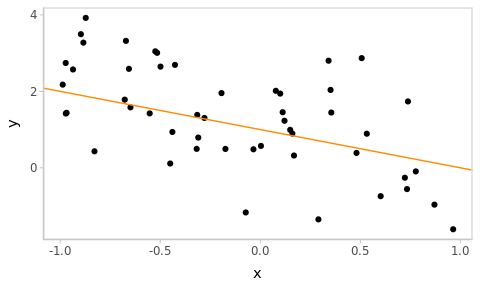
Figure 2.1: Simulated data with the true underlying relationship in orange.

2.1 Linear model

Fit the Linear Model (2.1) to the simulated data dat with:

fm_hw <- rstanarm::stan_glm(
  y ~ x, 
  data = dat
)

and obtain numerical and graphical summaries of the results using the generic R functions summary() and plot():

summary(fm_hw)
#> 
#> Model Info:
#>  function:     stan_glm
#>  family:       gaussian [identity]
#>  formula:      y ~ x
#>  algorithm:    sampling
#>  sample:       4000 (posterior sample size)
#>  priors:       see help('prior_summary')
#>  observations: 50
#>  predictors:   2
#> 
#> Estimates:
#>               mean   sd   10%   50%   90%
#> (Intercept)  1.1    0.2  0.9   1.1   1.3 
#> x           -1.4    0.3 -1.7  -1.4  -1.0 
#> sigma        1.1    0.1  1.0   1.1   1.3 
#> 
#> Fit Diagnostics:
#>            mean   sd   10%   50%   90%
#> mean_PPD 1.3    0.2  1.1   1.3   1.6  
#> 
#> The mean_ppd is the sample average posterior predictive distribution of the outcome variable (for details see help('summary.stanreg')).
#> 
#> MCMC diagnostics
#>               mcse Rhat n_eff
#> (Intercept)   0.0  1.0  3334 
#> x             0.0  1.0  3694 
#> sigma         0.0  1.0  3436 
#> mean_PPD      0.0  1.0  3670 
#> log-posterior 0.0  1.0  1765 
#> 
#> For each parameter, mcse is Monte Carlo standard error, n_eff is a crude measure of effective sample size, and Rhat is the potential scale reduction factor on split chains (at convergence Rhat=1).

# Equivalent to bayesplot::mcmc_intervals(fm_hw)
# See ?plot.stanreg for plotting options
plot(fm_hw)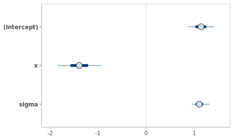

Congratulations!!! you have just fitted a Bayesian linear model!!

2.2 Inspecting results

Let’s fit the same model using a frequentist methodology. The code is essentially the same as before, just replacing the call to rstanarm::stan_glm() by stats::lm()¹.

fm_hw_lm <- lm(
  y ~ x, 
  data = dat
)

summary(fm_hw_lm)
#> 
#> Call:
#> lm(formula = y ~ x, data = dat)
#> 
#> Residuals:
#>     Min      1Q  Median      3Q     Max 
#> -2.4042 -0.7555 -0.1142  0.8879  2.4379 
#> 
#> Coefficients:
#>             Estimate Std. Error t value Pr(>|t|)    
#> (Intercept)   1.1361     0.1590   7.145 4.42e-09 ***
#> x            -1.3888     0.2712  -5.121 5.33e-06 ***
#> ---
#> Signif. codes:  0 '***' 0.001 '**' 0.01 '*' 0.05 '.' 0.1 ' ' 1
#> 
#> Residual standard error: 1.093 on 48 degrees of freedom
#> Multiple R-squared:  0.3533, Adjusted R-squared:  0.3399 
#> F-statistic: 26.23 on 1 and 48 DF,  p-value: 5.33e-06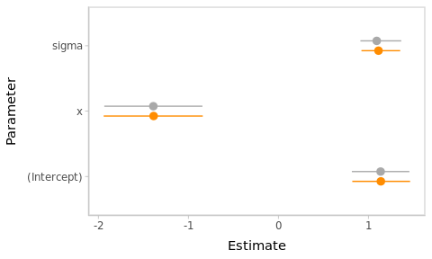

Figure 2.2: Frequentist and Bayesian point and interval estimates for the Hello World linear model.

The point and interval estimates of the model parameters (\(\beta_0\), \(\beta_x\) and \(\sigma\)) are compared in the Figure 2.2.²

The numerical estimates from both approaches are almost identical in this example. However, this will not always be the case. Besides, their interpretation is totally different, as we will see later.

To begin with, they are called differently:

Table 2.1: Nomenclature of point and interval estimates in the frequentist and the Bayesian frameworks.

Estimate	Frequentist	Bayesian
Point	Maximum-Likelihood	Posterior mean (or median, or…)
Interval	Confidence Interval	Credible Interval

2.3 In summary

• We fitted a Bayesian linear model using the package rstanarm to some simple simulated data

• It took nearly the same effort as the frequentist equivalent and gave nearly the same numerical results

• Yet, it seems that these results have different meaning and there is some prior thing for which we used a default specification.

• Pending questions: why bother if numerical results are similar; what is the role of the prior; how is the interpretation of the results different.

We will tackle the first two questions in the next section. But here is a teaser: numerical results are sometimes very different from frequentist outcomes, and this has everything to do with the priors.

3 Priors: contextualising data

Suppose that you are the head of a biological laboratory recently installed in a small village. While Covid’s positivity rate is currently very low (< 5%) overall in the country, out of your first 3 tests, 2 were positive for SARS-CoV-2.

pcr_dat <- data.frame(y = c(1, 1, 0))

Figure 3.1: 2 out of 3 patients in the sample tested positive.

Your assistant computes frequentist estimates for a proportion in order to estimate the positivity rate in the village and to test whether the observed data is consistent with the hypothesis of a positivity rate of 5%:

prop.test(x = sum(pcr_dat$y), n = nrow(pcr_dat), p = 0.05)
#> Warning in prop.test(x = sum(pcr_dat$y), n = nrow(pcr_dat), p = 0.05):
#> Chi-squared approximation may be incorrect
#> 
#>  1-sample proportions test with continuity correction
#> 
#> data:  sum(pcr_dat$y) out of nrow(pcr_dat), null probability 0.05
#> X-squared = 12.789, df = 1, p-value = 0.0003486
#> alternative hypothesis: true p is not equal to 0.05
#> 95 percent confidence interval:
#>  0.1253345 0.9823472
#> sample estimates:
#>         p 
#> 0.6666667

Horrified, he claims to have found that Covid’s positivity rate in the village is very likely above 10% (95% CI: [12-98]) and certainly (p < 0.001) above the global positivity rate of 5% and urges you to fire the epidemiological alarm.

What would you do?

More experienced, you calm him down and explain that the situation certainly deserves attention, but you need to collect more confirmatory evidence before panicking. Indeed,

• In a context of low epidemic transmission, a true high positivity rate in a small village would be very unlikely.

• Instead, other factors appear as more plausible explanations for the observations. Even if they are relatively unlikely themselves. E.g.,

  • Malfunctioning equipment
  • Human mistakes in the manipulation of the samples or the results
  • Patients might be relatives or have recently gathered (i.e. not a random, sample of independent test-users)

In a way, you are weighting the evidence in the observed data with your prior knowledge about the epidemiological situation. In the current context, a positivity rate of 66 % is very unlikely (i.e., incompatible with to your prior expectations), and extraordinary claims require extraordinary evidence.

Bayesian statistics allow to embed these considerations into the model, and to produce estimates given the available data and your prior expectations.

[Diagnostic tests example]

3.1 Logistic model

The model used in this case is a simple extension of the linear model (2.1) (i.e. a Generalized Linear Model, or GLM) where we replaced the Gaussian likelihood by a Binomial and there are no regression variables in the linear predictor.

Let \(Y\) be the number of positive tests in the sample of size \(n\),

\[\begin{align} Y & \sim \text{Bi}(n, \pi) \\ \eta & = \text{logit}(\pi) = \beta_0 \tag{3.1} \end{align}\] where \(\text{logit}(\pi) = \log(\pi / (1 - \pi))\).

The quantity of interest is the population’s positivity rate \(\pi \in (0, 1)\). However, the corresponding model parameter is \(\beta_0 \in \mathbb{R}\) (the intercept of the linear predictor) who varies in the logit scale.

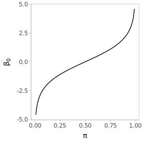
Figure 3.2: The logit transformation stretches the interval (0, 1) to the real line.

Let’s first verify that this model actually yields analogous estimates for the population positivity rate, using a frequentist procedure.

(
  fm_pcr_glm <- 
    glm(
      y ~ 1,
      family = binomial, 
      data = pcr_dat
    )
)
#> 
#> Call:  glm(formula = y ~ 1, family = binomial, data = pcr_dat)
#> 
#> Coefficients:
#> (Intercept)  
#>      0.6931  
#> 
#> Degrees of Freedom: 2 Total (i.e. Null);  2 Residual
#> Null Deviance:       3.819 
#> Residual Deviance: 3.819     AIC: 5.819

Only, the estimate is in logit scale and we have to transform the results, including the confidence interval, back to the original scale. How exactly to do that, is not important now (you can check the source code). Actually, there are several alternative methods leading to different results.

#> Warning: There was 1 warning in `mutate()`.
#> ℹ In argument: `across(.fns = plogis)`.
#> Caused by warning:
#> ! Using `across()` without supplying `.cols` was deprecated in dplyr 1.1.0.
#> ℹ Please supply `.cols` instead.

Table 3.1: Frequentist point and interval estimates of the population positivity rate in the PCR example.

term	estimate	conf.low	conf.high
\(\pi\)	0.67	0.16	0.98

While we obtained the same point estimate as with prop.test() (which is simply the sample proportion of positive tests), the lower end of the 95% Confidence Interval is somewhat higher. This is simply a consequence of the different procedures used for the computation of CIs in each case. Again, this is not very important at the moment.

However, what I want to establish is that this GLM essentially reproduces our initial estimates for the population positivity rate.

3.2 Prior elicitation

In order to fit the same model using a Bayesian approach, we want to encode our prior knowledge into a probability density for the model parameter \(\beta_0\).

This is not to mean that \(\beta_0\) is random in the sense that its value varies. However, we don’t know its actual value, and we are using a probability distribution to represent the available information about its value.

We know that the global population positivity rate is below 5%, and we would be very surprised that the true positivity rate in the village was larger than 50%. We can translate that knowledge into the following probability statements:

\[\begin{align} .50 & = P(\pi \leq .05) = P(\beta_0 \leq \text{logit}(.05)) \\ .99 & = P(\pi \leq .50) = P(\beta_0 \leq \text{logit}(.50)), \end{align}\] since \(\beta_0 = \text{logit}(\pi)\).

In other words, \(q_{.50} = \text{logit}(.05)\) and \(q_{.99} = \text{logit}(.50)\) are the \(.50\) and \(.99\) quantiles of \(\beta_0\)’s distribution. Note that quantiles are preserved under non-linear transformations.

If we consider a prior Gaussian distribution on \(\beta_0\) as \[\beta_0 \sim \mathcal{N}(\mu_0,\, \sigma_0), \] we just have to choose the values of \(\mu_0\) and \(\sigma_0\) that match the probability statements above.

3.2.1 Mathematical approach

Writing \(\beta_0 = \mu_0 + \sigma_0 \phi\), with \(\phi \sim \mathcal{N}(0, 1)\), we have \(q_\kappa = \mu_0 + \sigma_0 \Phi^{-1}(\kappa)\), where \(\Phi^{-1}\) is the quantile function of the standard normal distribution (a.k.a. the probit function).

Solving for \(\mu_0\) and \(\sigma_0\),

mu0 <- qlogis(.05)  # In R, qlogis() gives the logit function. See help.
s0 <- (qlogis(.50) - qlogis(.05)) / qnorm(.99)

\[\begin{align} \mu_0 & = q_{.50} = \text{logit}(.05) = -2.94 \\ \sigma_0 & = \Big(\text{logit}(.50) - \text{logit}(.05) \Big) / \Phi^{-1}(.99) = 1.27. \end{align}\]

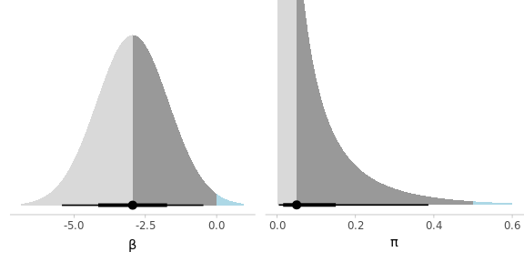
Figure 3.3: Elicited prior distribution for the model parameter and the implied prior on the positivity rate.

It is a good idea to visualize the implied prior in terms of the natural scale, for confirmation. Once we are satisfied with our probabilistic representation of our previous knowledge, we can proceed with the estimation.

This method of prior elicitation requires some mathematical skills. Furthermore, it exploits some specific properties of the Gaussian distribution. In more general and complex scenarios this approach might become unfeasible or impractical.

3.2.2 Computational approach

An alternative method is to take advantage of the computational capacity at our disposal and let the computer find the values for us. This is based on numerical optimisation and is completely general. Instead, it requires some programming skills in order to define custom functions.

## Quantile function for pi, given the prior parameters
qpi <- function(mu0, s0, p0) {
  setNames(
    plogis(qnorm(p = p0, mean = mu0, sd = s0)),
    paste0("q_", p0)
  )
}
# Verify that the prior paramters computed before yield the desired quantiles
# qpi(-2.94, 1.27, p0 = c(.5, .99))

## Target function to be optimised with respect to parameters
## Simply the sum of squared difference of the quantile function
## with respect to the target quantiles
target_pi <- function(par, p0, q0) {
  sum( (qpi(par[1], par[2], p0) - q0) ** 2 )
}
# target_pi(par = c(-4.6, 1.98), p0 = c(.5, .99), q0 = c(.01, .5))

## Call to R's general optimiser, to find the parameters that minimise
## the value of the target function.
(par0 <- optim(
  par = c(0, 1),   # initial values of parameters
  fn = target_pi,  # function to minimize with respect to the first argument
  p0 = c(.5, .99), # target cumulative probabilities
  q0 = c(.05, .5)  # target corresponding quantiles
))
#> $par
#> [1] -2.944555  1.265763
#> 
#> $value
#> [1] 1.894944e-10
#> 
#> $counts
#> function gradient 
#>       69       NA 
#> 
#> $convergence
#> [1] 0
#> 
#> $message
#> NULL

## Check
## Verify that the parameters found yield the required quantiles for pi
qpi(par0$par[1], par0$par[2], p0 = c(.5, .99))
#>     q_0.5    q_0.99 
#> 0.0499945 0.5000126

3.3 Results

We can now proceed to fit the model, including the elicited prior, to the data (Fig. 3.1).

pcr_prior_lowp <- normal(-2.94, 1.26)

fm1_pcr <- rstanarm::stan_glm(
  y ~ 1,
  family = binomial(),
  data = pcr_dat,
  prior_intercept = pcr_prior_lowp
)

The point and interval estimates of the positivity rate \(\pi\) from frequentist and Bayesian perspectives are displayed in Figure 3.4

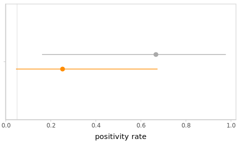
Figure 3.4: Frequentist and Bayesian point and interval estimates for the PCR example. The global positivity rate of 5% was added as a vertical line for reference.

3.4 Exercises

1. Match the priors

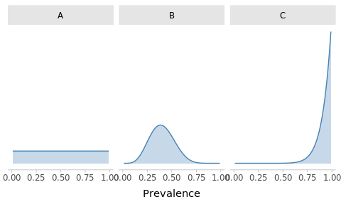
   Suppose that the government stopped monitoring SARS-CoV-2 (hypothetically) so you don’t have a reliable picture of the global situation. You consider 3 potential prior distributions for the prevalence:

   1. Optimistic: you are confident that the prevalence must be under control

   2. Clueless: you are unsure, anything is possible

   3. Conspiracist: despite the seeming normality, you beleive that the situation is dire

   Can you match the following plots with the priors?

   

2. High-prevalence context

   Suppose that you observed the same data but in a context where the global positivity rate is of about 50%, with a lot of variation across the territory (i.e. cases are concentrated on some specific regions).

   Change your prior accordingly and refit the model. How did conclusions change?

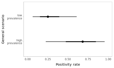
Figure 3.5: Estimated positivity rates depend on the context.

3. Larger sample size

   Suppose that the next day you tested 6 additional people, with the same proportion of positives (i.e. 4/6 positives). Aggregating the data from both days, obtain and compare the corresponding estimates for the positivity rate in the village under both scenarios.

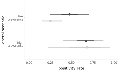
Figure 3.6: As more data is observed, the impact of the prior progressively fades away and estimates become more precise. Results from the previous ‘sparse’-data scenario are shown in light-grey for reference.

3.5 In summary

• The same data is (and should be) interpreted differently depending on the context.³

• This can be formalised by using prior distributions over the model parameters in a Bayesian framework.

• Bayesian statistics uses probability to represent information about things (e.g. model parameters).

• Priors are particularly important when observations are scarce, extreme, unexpected or uninformative. They work as a safety device.

• Conversely, the impact of the prior vanishes as the evidence accumulates. Regardless of prior beliefs, everyone reach to the same conclusions after observing sufficient data.

4 Posteriors: much more than point-and-interval estimation

In the same way as the prior distribution represents the information about a parameter before observing the data, the Bayesian model fit yields full posterior probability distributions for every parameter, representing the knowledge about the parameters after observing the data.

Rather than a mathematical expression for the posterior distribution, rstanarm yields a random sample from it, which can be summarized in different ways: posterior mean, median, mode, quantiles, credible intervals… or a summary plot of the posterior densities, as shown in Figure 4.1.

The function bayesplot::mcmc_areas() plots the posterior distributions of the parameters or any transformation of them.

plot_grid(
  mcmc_areas(fm1_pcr),  #  posterior for the (only) model parameter beta_0
  mcmc_areas(fm1_pcr, transformations = 'plogis')  # posterior for pi
)

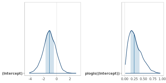
Figure 4.1: Posterior densities of the positivity rate in the logistic and natural scales. The vertical lines and bands represent the medians and the 50% central intervals respectively.

This is much more informative than simple point and interval estimates. Unlike frequentist Confidence Intervals, you can formulate all kind of probabilistic statements using the posterior distributions of the model parameters or their transformations.

For instance, what is the probability that the positivity rate \(\pi\) (a transformation of the model parameter \(\beta_0\)) exceeds 0.5, or is below 0.1…?

post_samples <- as.matrix(fm1_pcr)  # 4000 x 1 matrix with values from
                                    # the posterior distribution of beta_0
post_pi <- plogis(post_samples)     # posterior sample for pi

post_pi_below_50 <- mean(post_pi < .5)  # Proportion of values below 0.5

Despite your strong prior beliefs (\(P(\pi < 0.50) = 0.99\)), after looking at 3 observations, the posterior probability that the positivity rate in the village is below 0.5 dropped to \(P(\pi < 0.50 \,|\, \text{Data}) = 0.88\).

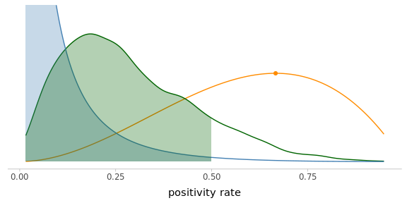
Figure 4.2: The posterior distribution is making a compromise between your prior knowledge and the evidence from the observed data (scaled likelihood).

Check out the excellent interactive visualisation by Kristoffer Magnuson, to illustrate the interplay between these three components of Bayesian inference.

4.1 Exercises

1. Using the previous interactive visualisation tool, determine in which situations the posterior distribution closely matches the likelihood, regardless of the effect size.

2. Compute the posterior probabilities that the positivity rate in the village is below 0.5 under the high-prevalence and the larger sample size scenarios from the previous section.

   Table 4.1 displays the results I obtained. Discuss and explain the differences between posterior probabilities across scenarios.

   Table 4.1: Posterior probability that the positivity rate is below 50% depending on the scenario (global context and sample size), for the same proportion (2/3) of observed positives.

   	Context
   Sample size	Low-prevalence	High-prevalence
   3	0.88	0.28
   9	0.57	0.14

4.2 In summary

• The resulting inference about model parameters (or any transformation of them) is encoded in posterior probability density functions (or, rather, a random sample from them) which can be summarized in different ways for communication purposes.

• Credible Intervals can be interpreted in probabilistic terms.

• Posterior distributions are a trade-off between prior information and evidence from the observed data. Strong priors and sparse data result in little learning, whereas weaker priors have negligible impact in the presence of abundant data.

5 Comparison of group means

Comparing average expected outcomes of different groups is a typical goal in experimental settings (e.g. control and treatment groups), for which several frequentist approaches are commonly used (t-tests, ANOVA, ANCOVA…). Essentially, all these reduce to a linear model with one or more categorical factors.

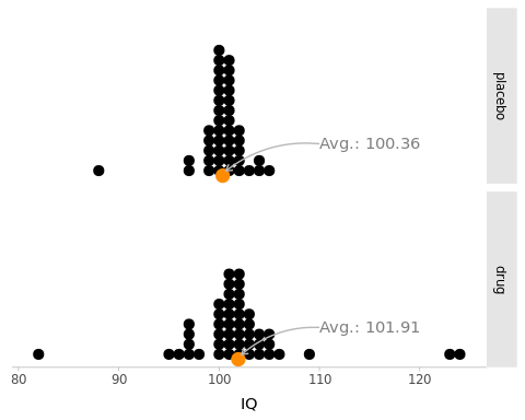
Figure 5.1: Simulated scores from two randomized groups of people: ‘drug’ (\(N_1 = 47\)) and ‘placebo’ (\(N_2 = 42\)) who take an IQ test. The sample averages are represented by an orange point at the bottom.

The data represented in Figure 5.1 is extracted from Kruschke (2013) and is included in crashbayes as best.

The average IQ score in the drug group is slightly larger than that of the placebo group. But the difference is relatively small with respect to the individual variation within groups.

The question is classically framed in terms of whether the drug has any significant effect.⁴ This is a bit confusing, because it does not tell much about what we typically want to know (Greenland et al. 2016; Gelman 2013).

Instead, we are going to assess the relative credibility of the possible values of the effect with a posterior probability distribution.

Let’s start by assuming a tentative model for the data. A linear model (which is the model behind the \(t\)-test) is a good starting point.

\[\begin{align} Y_i & \sim \mathcal{N}(\mu_i, \sigma) \\ \mu_i & = \beta_0 + \beta_\text{d} \mathbb{1}_\text{d}[i] \tag{5.1} \end{align}\] where \(i\) is the group (drug, or placebo), and \(\mathbb{1}_\text{d}[i]\) evaluates to 1 when the observation belongs to the drug group and to 0 otherwise.

The effect of the drug is \(\beta_\text{d}\). But the model also involves the parameter \(\beta_0\) (the expected value of the placebo group) and \(\sigma\) the individual standard-deviation of values within both groups.

5.1 Using default priors

The authors of rstanarm (Goodrich and Gabry 2020) have put a lot of thought and effort on coming up with reasonable default priors.

Let’s start from there and adjust later.

fm0_best <- rstanarm::stan_glm(
  y ~ 1 + group,
  family = gaussian(),  # Default, but making it explicit.
  data = best
)

Function summary() can be used on a fitted model in order to obtain summary and diagnostic statistics. We can directly obtain point and interval numerical estimates for the target effect groupdrug.

summary(fm0_best)
#> 
#> Model Info:
#>  function:     stan_glm
#>  family:       gaussian [identity]
#>  formula:      y ~ 1 + group
#>  algorithm:    sampling
#>  sample:       4000 (posterior sample size)
#>  priors:       see help('prior_summary')
#>  observations: 89
#>  predictors:   2
#> 
#> Estimates:
#>               mean   sd    10%   50%   90%
#> (Intercept) 100.4    0.7  99.4 100.3 101.3
#> groupdrug     1.6    1.0   0.3   1.6   2.8
#> sigma         4.7    0.3   4.3   4.7   5.2
#> 
#> Fit Diagnostics:
#>            mean   sd    10%   50%   90%
#> mean_PPD 101.2    0.7 100.3 101.2 102.1
#> 
#> The mean_ppd is the sample average posterior predictive distribution of the outcome variable (for details see help('summary.stanreg')).
#> 
#> MCMC diagnostics
#>               mcse Rhat n_eff
#> (Intercept)   0.0  1.0  4185 
#> groupdrug     0.0  1.0  4337 
#> sigma         0.0  1.0  3589 
#> mean_PPD      0.0  1.0  4046 
#> log-posterior 0.0  1.0  1656 
#> 
#> For each parameter, mcse is Monte Carlo standard error, n_eff is a crude measure of effective sample size, and Rhat is the potential scale reduction factor on split chains (at convergence Rhat=1).

We can specify optional arguments to the plot() function in order to focus on the target parameter \(\beta_\text{d}\) and to display the full posterior probability density rather than the default point-interval summary in figure 5.2.

plot(fm0_best, plotfun = 'areas', pars = 'groupdrug')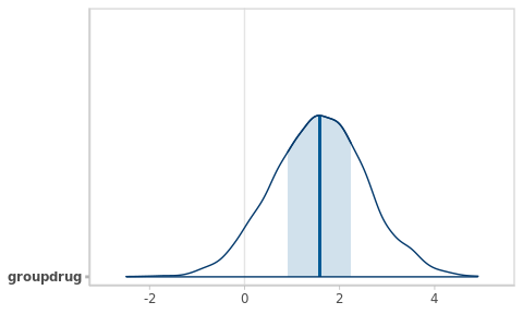

Figure 5.2: Posterior density function for the target parameter.

Finally, we can extract a sample from the posterior distribution and compute, for instance, the probability that the effect is positive by computing the corresponding proportion.

(post_drug_gt0 <- mean(as.matrix(fm0_best)[, "groupdrug"] > 0))
#> [1] 0.943

Note that this effect would be considered not significant under a classical approach:

fm0_best_freq <- lm(y ~ group, data = best)
summary(fm0_best_freq)
#> 
#> Call:
#> lm(formula = y ~ group, data = best)
#> 
#> Residuals:
#>      Min       1Q   Median       3Q      Max 
#> -19.9149  -0.9149   0.0851   1.0851  22.0851 
#> 
#> Coefficients:
#>             Estimate Std. Error t value Pr(>|t|)    
#> (Intercept) 100.3571     0.7263 138.184   <2e-16 ***
#> groupdrug     1.5578     0.9994   1.559    0.123    
#> ---
#> Signif. codes:  0 '***' 0.001 '**' 0.01 '*' 0.05 '.' 0.1 ' ' 1
#> 
#> Residual standard error: 4.707 on 87 degrees of freedom
#> Multiple R-squared:  0.02717,    Adjusted R-squared:  0.01599 
#> F-statistic:  2.43 on 1 and 87 DF,  p-value: 0.1227
confint(fm0_best_freq)
#>                 2.5 %     97.5 %
#> (Intercept) 98.913627 101.800658
#> groupdrug   -0.428653   3.544155

We can check which priors were used in a given model using the function prior_summary()

prior_summary(fm0_best)
#> Priors for model 'fm0_best' 
#> ------
#> Intercept (after predictors centered)
#>   Specified prior:
#>     ~ normal(location = 101, scale = 2.5)
#>   Adjusted prior:
#>     ~ normal(location = 101, scale = 12)
#> 
#> Coefficients
#>   Specified prior:
#>     ~ normal(location = 0, scale = 2.5)
#>   Adjusted prior:
#>     ~ normal(location = 0, scale = 24)
#> 
#> Auxiliary (sigma)
#>   Specified prior:
#>     ~ exponential(rate = 1)
#>   Adjusted prior:
#>     ~ exponential(rate = 0.21)
#> ------
#> See help('prior_summary.stanreg') for more details

Here we can see:

• A different prior for each of the three parameters in the model

• Each of these default priors has been adjusted to match the scale of the observed data⁵

• The prior intercept is centred at the average response in the dataset

• The prior intercept is applied to a (internally) re-parametrised model, where all the predictors are centred.

  This is very useful for continuous covariates, because the intercept represents the expected outcome at the average value of \(x\) rather than at \(x = 0\). But less so in this case, where the expected outcome of the placebo group is more meaningful than the expected average outcome, which depends essentially on the number of observations that we happened to have on each group.

  As explained in rstanarm’s documentation on prior distributions, we can disable this by manually creating a intercept variable or by using an option for sparse computation (see next).

5.2 Specifying custom priors

A little domain knowledge tells us that IQ tests are designed to have a median of 100 and a standard deviation of 15. This is very valuable information for specifying priors for \(\beta_0\) and \(\sigma\). For instance, we could propose:

\[ \begin{aligned} \beta_0 & \sim \mathcal{N}(100, 5) \\ \beta_\text{d} & \sim \mathcal{N}(0, s_0) \\ \sigma & \sim \text{Exp}(1/15) \end{aligned} \]

Regarding the target parameter \(\beta_\text{d}\), we don’t expect the drug to turn a a average IQ (90-109) into a very superior one (130+). Thus, we can assume that the effect of the drug is almost surely below 30.

## Find the Gaussian SD that yields a cumulative probability of
## .9986 at x = 45
cump <- function(x) pnorm(30, mean = 0, sd = x)
target <- function(x) (cump(x) - .999)**2
(s0 <- optimise(target, interval = c(0, 20))$minimum)
#> [1] 9.708007

best_prior_b0 <- normal(100, 5)
best_prior_sigma <- exponential(1/15)
best_prior_bdrug <- normal(0, s0)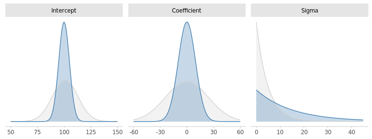

Figure 5.3: Default and custom priors for the model paramters.

Our custom priors are rather consistent with the default ones, albeit somewhat more informative. With the exception of \(\sigma\). Any thoughts about that?

We will come back to \(\sigma\) later. Let’s first fit the model to the data using our carefully crafted priors.

fm1_best <- rstanarm::stan_glm(
  y ~ 1 + group,
  family = gaussian(),
  data = best,
  prior_intercept = best_prior_b0,
  prior           = best_prior_bdrug,
  prior_aux       = best_prior_sigma,
  sparse = TRUE   ## Disables "centering" of predictors
)

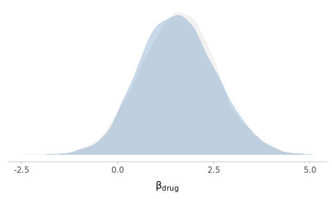
Figure 5.4: Posterior density estimates of the drug effect using default and custom priors.

As you can see, despite the relatively important differences in the prior specifications, the results are essentially identical. Why do you think this is the case?

5.3 In summary

• Bayesian estimation yields much richer information about group differences (or any model parameter) than the classical counterparts. There is literally no reason to continue performing \(t\)-tests (or ANOVA) nowadays (Kruschke 2013).

• But we are not done yet. Before trusting these results we need to perform some checks and validations.

6 Model assessment

6.1 MCMC diagnostics

The last section of the summary() reports some basic diagnostic values for each parameter in the model.

summary(fm1_best)
#> 
#> Model Info:
#>  function:     stan_glm
#>  family:       gaussian [identity]
#>  formula:      y ~ 1 + group
#>  algorithm:    sampling
#>  sample:       4000 (posterior sample size)
#>  priors:       see help('prior_summary')
#>  observations: 89
#>  predictors:   2
#> 
#> Estimates:
#>               mean   sd    10%   50%   90%
#> (Intercept) 100.4    0.7  99.4 100.4 101.3
#> groupdrug     1.6    1.0   0.3   1.5   2.8
#> sigma         4.8    0.4   4.3   4.7   5.2
#> 
#> Fit Diagnostics:
#>            mean   sd    10%   50%   90%
#> mean_PPD 101.2    0.7 100.3 101.2 102.1
#> 
#> The mean_ppd is the sample average posterior predictive distribution of the outcome variable (for details see help('summary.stanreg')).
#> 
#> MCMC diagnostics
#>               mcse Rhat n_eff
#> (Intercept)   0.0  1.0  1791 
#> groupdrug     0.0  1.0  1860 
#> sigma         0.0  1.0  2556 
#> mean_PPD      0.0  1.0  3158 
#> log-posterior 0.0  1.0  1535 
#> 
#> For each parameter, mcse is Monte Carlo standard error, n_eff is a crude measure of effective sample size, and Rhat is the potential scale reduction factor on split chains (at convergence Rhat=1).

The text at the end of the summary provides some very succinct information for their interpretation. Essentially,

• mcse the Monte Carlo standard error is the error in estimates due to computing them from finite samples. Obviously, the smaller the better. But any magnitude under the practical resolution will suffice.

• Rhat is a technical measure of the convergence of the chains. It essentially evaluates whether estimates computed from the different chains are similar (which is why 4 chains are computed independently). It should be close to 1 (ideally, \(\pm\) 0.01, but \(\pm\) 0.1 is often sufficient).

• n_eff is a measure of effective sample size (ESS). Can be interpreted as the amount of information in the simulation in terms of a equivalent number of independent draws. The higher the better.

See the documentation on Runtime warnings and convergence problems for more details.

6.2 Posterior predictive checks

The results of a statistical analysis are conditional to the model, i.e., are only meaningful as long as the model is true. Or, more pragmatically, if the model is a reasonable approximation to the real data-generating process.

This is classically performed by examining various diagnostic plots, such as histograms of residuals or scatter plots of predicted values and observed data.

In a Bayesian setting, we get full posterior predictive distributions for the outcomes, which combine the uncertainties in the model parameters with the variability of the likelihood.⁶

We can use this posterior predictive distributions to simulate new outcomes and compare them to the actual observed dataset in various ways (Gabry et al. 2018).

We can use rstanarm::pp_check() with various options for examining the posterior predictive distributions from different angles.

pp_check(fm1_best, plotfun = 'dens')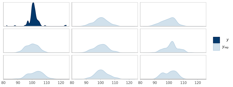

Figure 6.1: Empirical density of the observed outcomes (y) and the corresponding densities from 8 replicates from the fitted model.

It looks like the overall shape of the replicated outcomes is rather different from the actual values.

However, 8 replications are too few to get a reliable sense of the variation. Let’s overlay a few more, while splitting groups at the same time.

pp_check(fm1_best, plotfun = 'dens_overlay_grouped', group = 'group')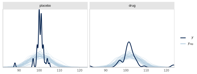

Figure 6.2: Empirical density of the observed outcomes (y) split by group and the corresponding densities from 100 replicates from the fitted model.

We can also compare the distribution of some summary statistic of the replicated data with the realised statistic for the observed data.

This helps us to challenge our current model and identify in which ways it does not accurately reproduce the patterns in the data.

The default statistic is the sample average (Fig. 6.3). The posterior predictive distribution of this statistic is summarised as mean_PPD, in the output of summary().

pp_check(fm1_best, plotfun = 'stat')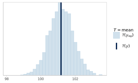

Figure 6.3: Posterior predictive check for the sample average.

As expected, simulating new data from the fitted model yields virtual samples with averages that vary around the observed average.

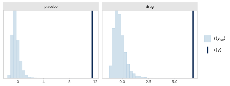
From the previous plots and the observation that the default prior for \(\sigma\) (based on the scale of the data) was narrower than our prior expectations, we can be interested in looking at the kurtosis and the standard deviation of the data.

## Compute the kurtosis of a sample x
kurtosis <- function(x) {
  m4 <- mean((x - mean(x)) ^ 4)
  kurtosis <- m4 / (sd(x) ^ 4) - 3
  kurtosis
}

pp_check(
  fm1_best,
  plotfun = 'stat_grouped',
  stat = kurtosis,
  group = 'group'
)

pp_check(
  fm1_best,
  plotfun = 'stat_grouped',
  stat = sd,
  group = 'group'
)

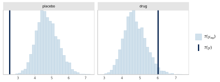
The model seems to be failing at reproducing the outliers in the data. And somewhat compensating with increased SD, specially in the placebo group. Besides, the dispersions within groups should probably be allowed to be different.

6.3 In summary

• Using posterior predictive checks, we identified 2 issues in the model specification: the dispersion of the outcomes should probably be different in each group and the Gaussian likelihood is not appropriate due to more extreme observations than what would be expected from a Gaussian distribution.

• Addressing these issues is straightforward in principle. We would simply replace the Gaussian likelihood by a Student-\(t\) and using a different parameter for the standard deviation in each group. However, such a Student likelihood is not built into rstanarm.

  We could instead specify this model in brms (Bürkner 2017) or in Stan directly, which are each more flexible and powerful, but require compilation of the model and different syntax. Not particularly difficult, but it’s an additional layer that I didn’t want to introduce today. I have left the code in the source file if you are curious.

7 Conclusions

• Given sufficiently informative data, the influence of the prior is negligible and both frequentist and Bayesian approaches give similar numerical point and interval estimates.

• Using priors can be crucial for: combining prior information with new evidence to progressively update scientific knowledge using solid probabilistic foundations; obtain valid results even with only sparse data is available; avoid numerical issues of multi-collinearity or divergences.

• Bayesian results have natural and straightforward interpretations in terms of probabilities, which represent the knowledge and the uncertainties about quantities of interest.

• Using rstanarm::stan_glm() and rstanarm::stan_glmer() you can effectively and easily fit Bayesian LMs, GLMs and GLMMs. This should cover most of your regression modelling needs, with with the additional benefits of using priors as a safety guard against over-fitting and posteriors for straightforward interpretation of results and for model evaluation.

• With a little bit more experience and training you can unlock brms and rstan for additional modelling flexibility. They require some more technical knowledge. However, the fundamental concepts and workflow for Bayesian analysis remain the same.

Bibliography

Bürkner, Paul-Christian. 2017. “Brms : An R Package for Bayesian Multilevel Models Using Stan.” Journal of Statistical Software 80 (1). https://doi.org/10.18637/jss.v080.i01.

Gabry, Jonah, and Tristan Mahr. 2022. Bayesplot: Plotting for Bayesian Models (version R package version 1.10.0). https://mc-stan.org/bayesplot/.

Gabry, Jonah, Daniel Simpson, Aki Vehtari, Michael Betancourt, and Andrew Gelman. 2018. “Visualization in Bayesian Workflow.” http://arxiv.org/abs/1709.01449.

Gelman, Andrew. 2013. “P Values and Statistical Practice.” Epidemiology 24 (1): 69–72. https://doi.org/10.1097/ede.0b013e31827886f7.

Goodrich, Ben, and Jonah Gabry. 2020. Rstanarm: Bayesian Applied Regression Modeling via Stan. (version R package version 2.21.1). https://mc-stan.org/rstanarm.

Greenland, Sander, Stephen J. Senn, Kenneth J. Rothman, John B. Carlin, Charles Poole, Steven N. Goodman, and Douglas G. Altman. 2016. “Statistical Tests, P Values, Confidence Intervals, and Power: A Guide to Misinterpretations.” European Journal of Epidemiology 31 (4): 337–50. https://doi.org/10.1007/s10654-016-0149-3.

Kruschke, John K. 2013. “Bayesian Estimation Supersedes the T Test.” Journal of Experimental Psychology. General 142 (2): 573–603. https://doi.org/10.1037/a0029146.

Siegfried, Tom. 2010. “Odds Are, It’s Wrong: Science Fails to Face the Shortcomings of Statistics.” Science News 177 (7): 26–29. https://doi.org/10.1002/scin.5591770721.