spreadrate

The goal of spreadrate is to estimate the local velocity of propagation of an epidemic event, given dates and locations of observed cases.

The method estimates the surface of first date of invasion by interpolation of the earliest observations in a neighbourhood and derives the local spread rate as the inverse slope of the surface.

Furthermore, it helps to quantify the estimation uncertainty by a Monte Carlo approach. Visualise and simulate the spatio-temporal progress of epidemics.

Installation

To install the latest version of spreadrate, copy and paste the following in a R session.

if (!require("remotes")) {
  install.packages("remotes")
}
install.packages("INLA", repos="https://inla.r-inla-download.org/R/testing")
remotes::install_gitlab("umr-astre/spreadrate", host = "forgemia.inra.fr")

Example

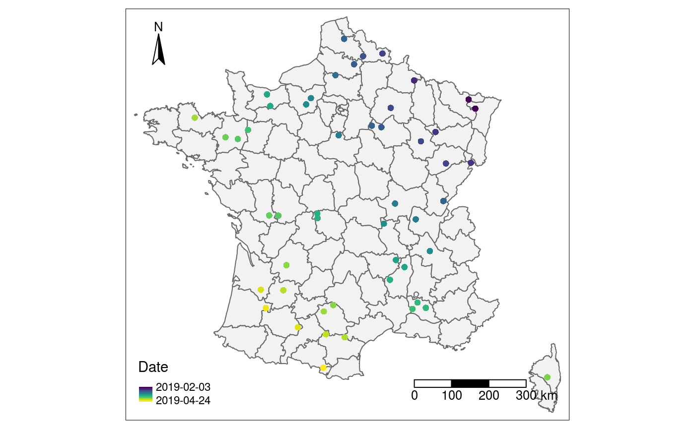
Suppose that we have recorded the GPS coordinates and observation dates for all the observed cases of some emerging disease in mainland France into a table like this one.

#> # A tibble: 50 x 3
#>    date         Lon   Lat
#>    <date>     <dbl> <dbl>
#>  1 2019-02-03  7.05  49.0
#>  2 2019-02-03  7.27  48.8
#>  3 2019-02-12  5.07  49.5
#>  4 2019-02-15  5.79  48.3
#>  5 2019-02-16  7.01  47.5
#>  6 2019-02-18  3.90  50.2
#>  7 2019-02-19  6.12  47.5
#>  8 2019-02-20  5.25  48.1
#>  9 2019-02-21  4.18  48.9
#> 10 2019-02-24  3.17  50.1
#> # … with 40 more rows

Here is a visual representation of these observed cases.

First let spreadrate interpret the observational data appropriately with the function sr_obs(). You need to specify the name of the temporal variable. Lon and Lat are recognised automatically.

library(spreadrate)
#> Loading required package: raster
#> Loading required package: sp
#> 
#> Attaching package: 'raster'
#> The following object is masked from 'package:dplyr':
#> 
#>     select
#> The following object is masked from 'package:tidyr':
#> 
#>     extract
cases_sr <- sr_obs(cases, "date")

However, spread-rate calculations require projected (rather than geographic) coordinates. An appropriate projection for mainland France is EPSG:2154. See https://epsg.io/.

cases_sr <- st_transform(cases_sr, crs = 2154)

Everything is now set to perform a default estimation of spread-rate.

sr_est <- sr(cases_sr)

Done! Here is a quick plot of the estimated local spread-rate. The estimated velocity is practically constant, between 9 and 11 km / day.

plot(sr_est, col = hcl.colors(12))

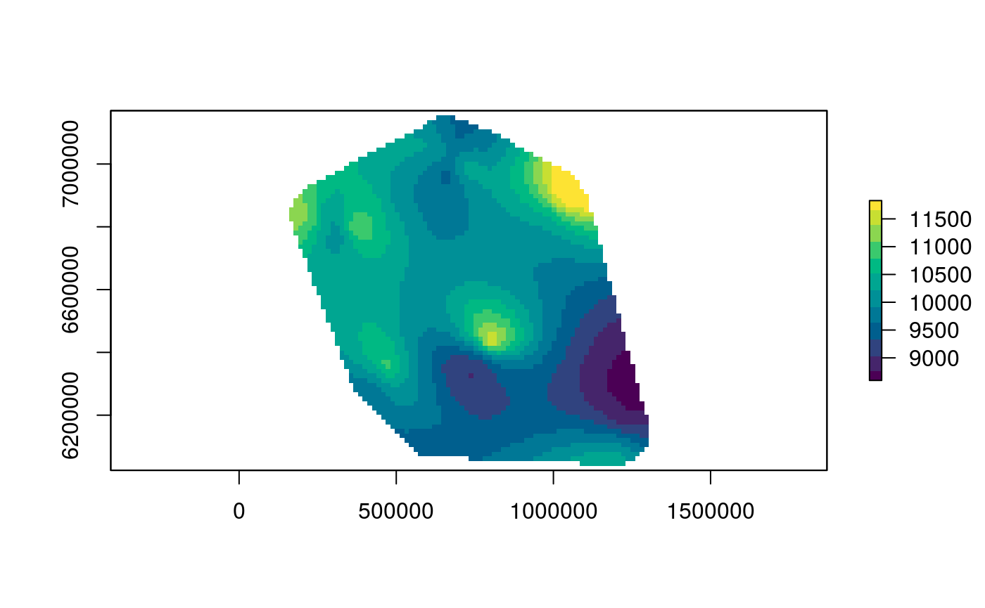
This is consistent with the value of 10^{4} m/day used for simulating the data.

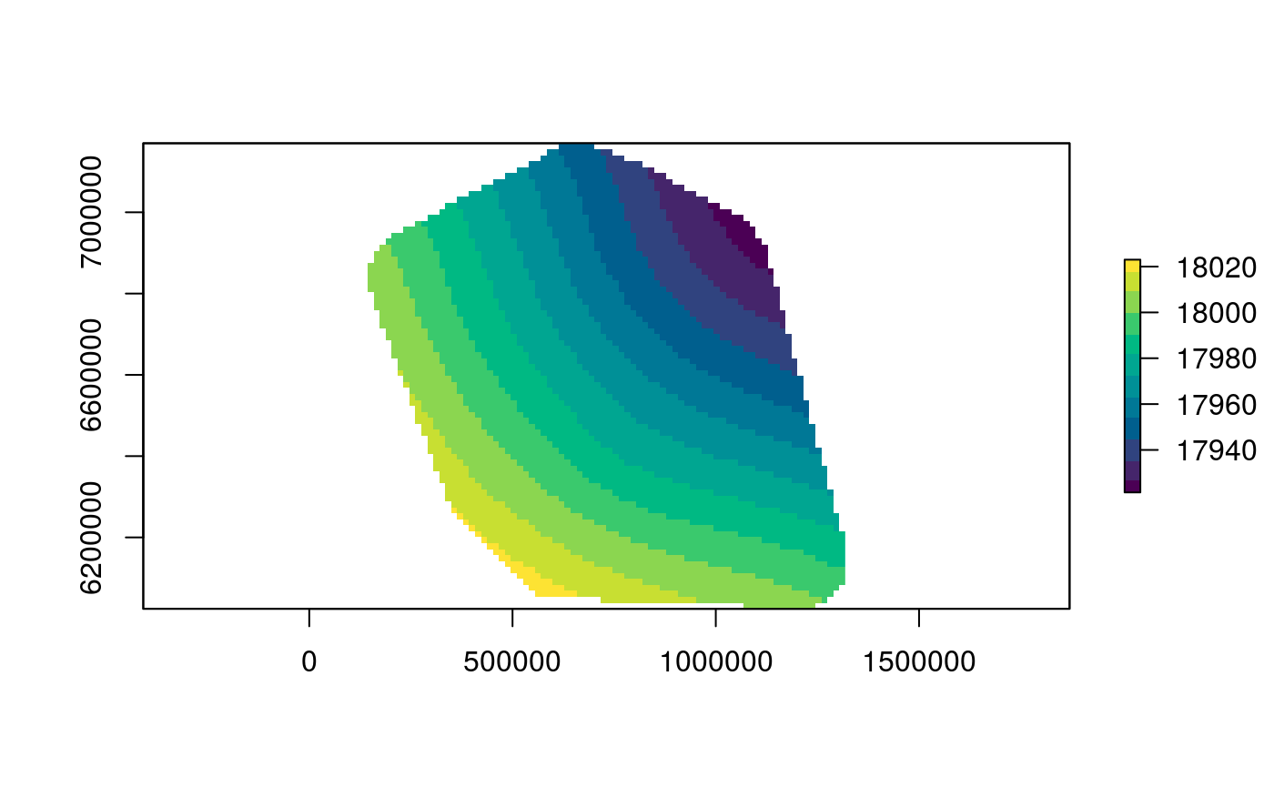
We can also retrieve the estimated surface of first-date of invasion:

plot(attr(sr_est, "fdoi"), col = hcl.colors(12))

References

Tisseuil, Clément, Aiko Gryspeirt, Renaud Lancelot, Maryline Pioz, Andrew Liebhold, and Marius Gilbert (2016). Evaluating Methods to Quantify Spatial Variation in the Velocity of Biological Invasions. Ecography 39, no. 5: 409–418. https://doi.org/10.1111/ecog.01393.