Getting Started
2024-03-19
mapMCDA.Rmd## Loading required package: sf## Linking to GEOS 3.10.2, GDAL 3.4.1, PROJ 8.2.1; sf_use_s2() is TRUE## Loading required package: terra## terra 1.7.65## Loading required package: mapMCDAIntroduction
The mapMCDA package facilitates the weighting of several
risk factors to produce an epidemiological risk map.
However, a user’s expertise can be crucial to the interpretation of
each risk factor. This is expressed at three levels within
mapMCDA:
Choice of relevant risk factors.
For each factor, setting a common risk scale (e.g. between 0 and 100).
Two-way assessment of the relative importance of the risk factors.
Next, we use the maps provided by the package to produce an example risk map. This map has no epidemiological value.
1. Risk factors
The function mapMCDA_datasets() is used to load into
memory all the maps available within the package.
The cmr object is a simple list of maps: objects of type
sf for vectorial for vector maps and of type
SpatRaster for raster maps.
To use other maps, use the functions sf::st_read and
terra::rast() for vector and raster maps respectively.
You can also use the load_layer() function to load any
type of maps automatically, as demonstrated in the commented code.
cmr <- mapMCDA_datasets()

# layers <- list.files(
#   system.file("cartography/CMR", package = "mapMCDA"),
#   full.names = TRUE
# )
# cmr <- lapply(layers, load_layer)
# names(cmr) <- rmext(basename(layers)))
One of these maps is that of the epidemiological units, used to establish the working framework.
epi_units <- cmr$cmr_admin3
par(mar = c(0, 0, 0, 0))
plot(st_geometry(epi_units))
Epidemiological units example for Cameroon.
2. Scaling
Each risk factor varies on its own scale. Animal density, for example, varies between 0 and almost 5500 heads per \(km^2\).
For vector maps, which show the location of spatial features such as lakes or forests, we consider the distance to these entities.
This package currently uses a linear function for scaling. However, the relationship can be direct or inverse.
plot(
  data.frame(x = c(0, 100), y = c(0, 100)),
  type = 'l',
  xaxs = "i",
  yaxs = "i",
  xaxt = "n",
  lab = c(1, 1, 7),
  xlab = c("Original scale"),
  ylab = c("Scale of risk")
)
abline(100, -1)
Direct or inverse scaling.
The risk_layer() function calculates the risk map
associated in a factor with a given scale. The default value is between
0 and 100. To reverse the relationship, simply pass the limits in
reverse order, e.g. c(100, 0).
Moreover, it uses the map of epidemiological units to establish risk calculation limits.
risks <- list(
  animal_density = risk_layer(
    cmr$animal.density,
    boundaries = epi_units
  ),
  water_bodies = risk_layer(
    cmr$water_bodies,
    boundaries = epi_units,
    scale_target = c(100, 0)  # renversed scale
  ),
  parks = risk_layer(
    cmr$national_parks,
    boundaries = epi_units,
    scale_target = c(100, 0)  # renversed scale
  )
)
##
|---------|---------|---------|---------|
=========================================
|---------|---------|---------|---------|
=========================================
We would like to examine the risk maps calculated in this way. But to do this, they need to be aligned. In other words, they must have the same extents, resolutions and projections.
We can use the align_layers() function, which arranges
all this for us. Note that this step is not necessary to continue, as
this function is automatically executed if necessary.
aligned_risks <- align_layers(risks)
plot(terra::rast(aligned_risks), nc = 3, col = grDevices::hcl.colors(50))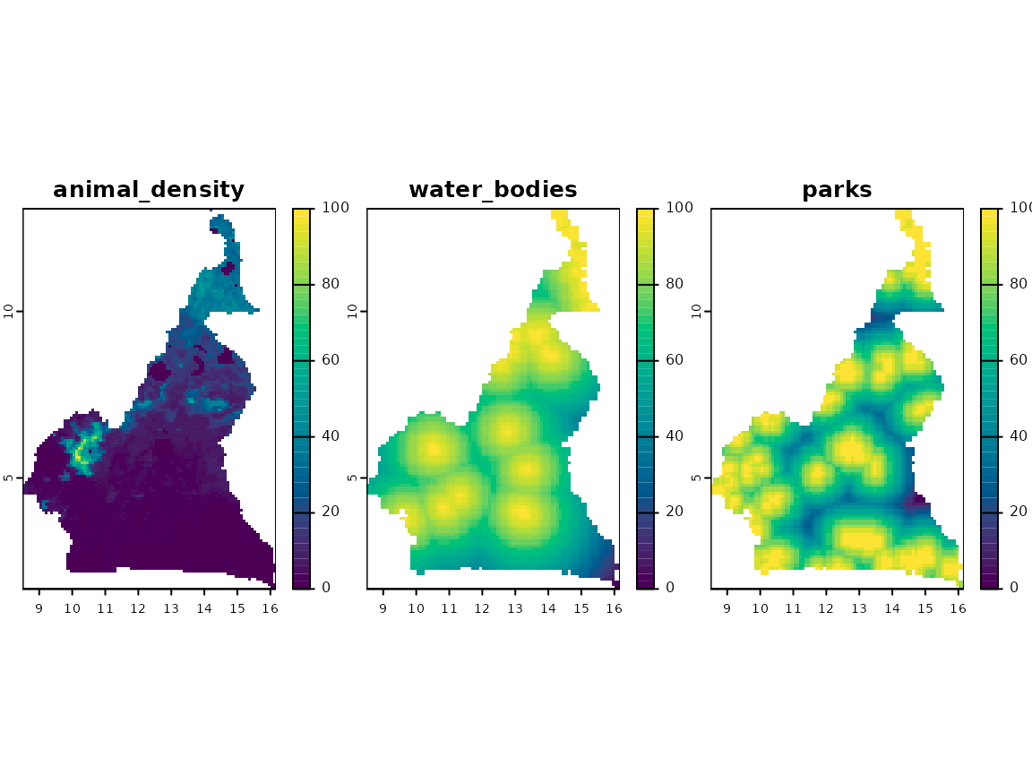
Level of risk associated with each risk factor.
3. Weighting of risk factors
There are three factors to consider. We need to compare their relative importance 2-by-2 on a scale of 1 to 9 and represent these relationships in a matrix which must have 1’s on its diagonal.
Note that symmetrical elements must be reciprocal.
| animal_density | water_bodies | parks | |
|---|---|---|---|
| animal_density | 1.00 | 6.00 | 4 |
| water_bodies | 0.17 | 1.00 | 3 |
| parks | 0.25 | 0.33 | 1 |
In this example, we consider that animal density is 6 times more important than the distance to watering holes, and 4 times more important than the distance to parks. At the same time, the distance to water points is 3 times greater than the distance to parks.
The system calculates the weighting coefficients that are most
consistent with these pairwise values, using the
compute_weights() function.
w <- compute_weights(M)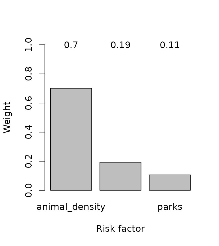
Weighting of risk factors.
4. Calculation of the risk map
The wlc() function (for weighted linear combination)
combines all the risk factors risk factors using the weights calculated
above, and produces a risk map covering the whole region.
combined_risk <- wlc(risks, w)
plot(combined_risk, col = hcl.colors(50))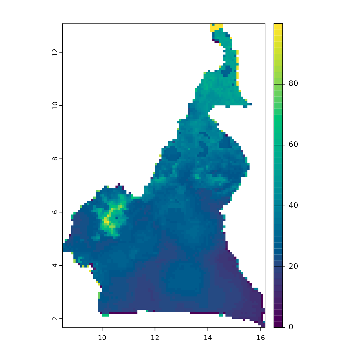
Map of combined risks.
Finally, a map can be produced for each epidemiological unit on a homogenized scale of risk.
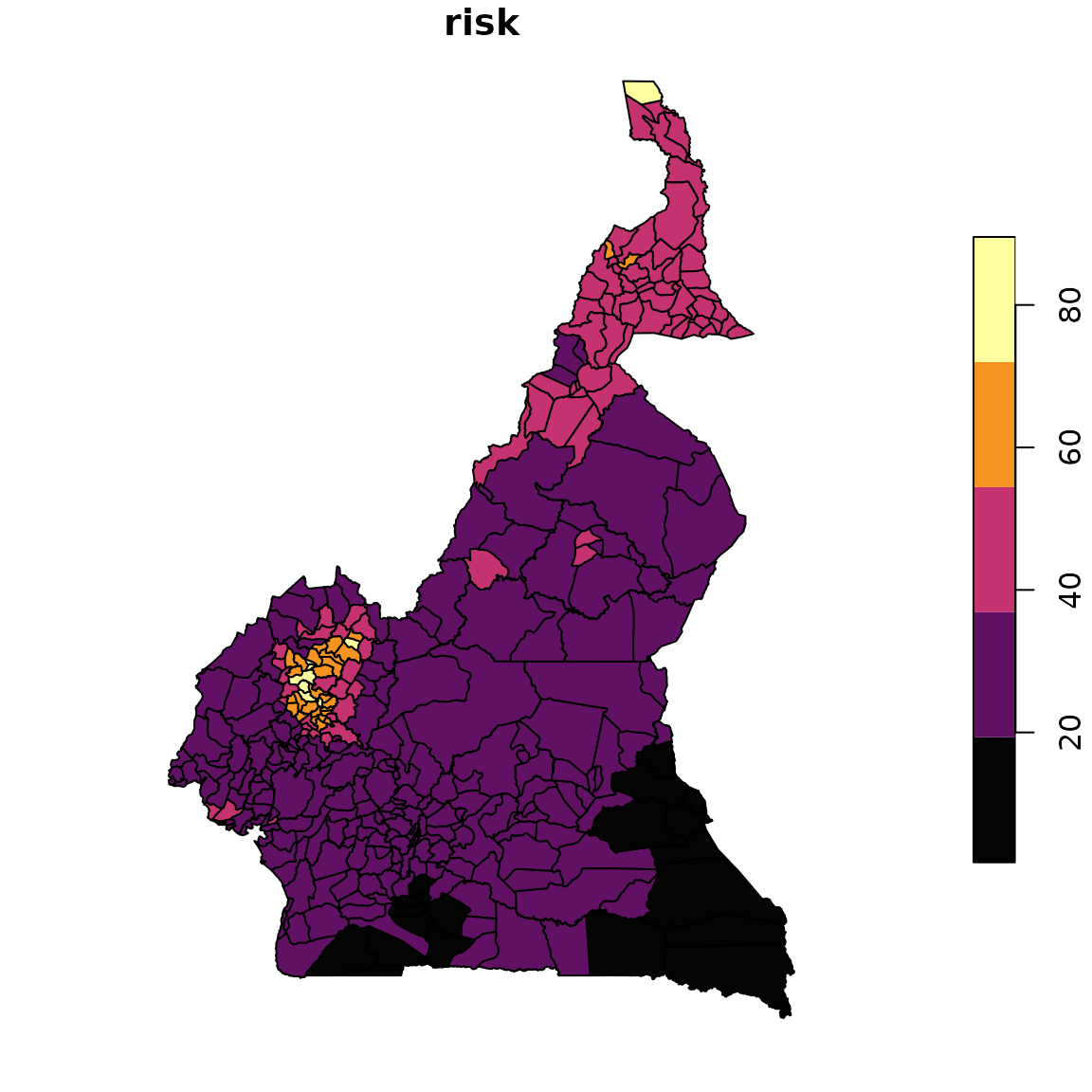
Map of risk level per epidemiological unit.